Reducing the Amount of Solution Data Stored in a Model
File sizes can become significant when a lot of solution data is generated. This is especially true for time-dependent models, but also for models involving parameter and frequency sweeps. In COMSOL Multiphysics®, there are several ways to keep your model sizes from becoming too large and taking up disk space. Here, we will discuss the different approaches for accomplishing this and showcase the features involved in each approach.
Using Probes for Time-Dependent Models
For many transient simulations, you may only be interested in some global quantities or the average, integral, maximum, or minimum quantities evaluated over some domains, boundaries, edges, or points. In cases like these, you can use probes.
After defining any probe(s) in your model for the quantities of interest and in the regions of interest of your model, you can then specify just the start time and end time in the Output times field in the Time Dependent study step Settings window. Doing so results in the field solutions only being saved at the start and end times. By default, the probes that you set up will still be updated and stored at all of the timesteps taken by the solver.
This will greatly reduce the amount of data in your model and can speed up solution time, especially in contrast to a model where data is being written out at many timesteps. Note that reducing the number of timesteps stored in output has no effect on the accuracy of the solution. This is described in our knowledge base entry on controlling the Time-Dependent Solver timesteps.
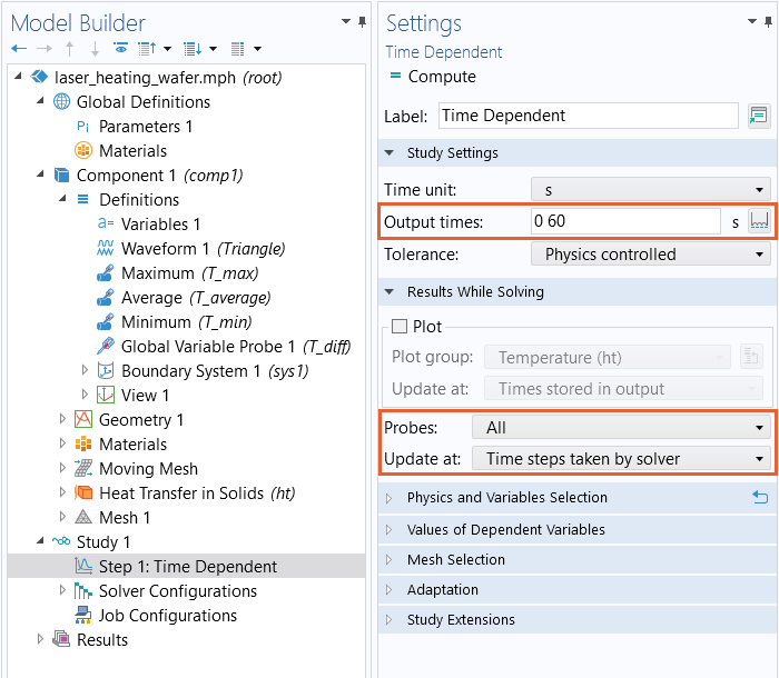 The start and end times specified in the settings of the Time Dependent study step. The default settings for the probes in the study settings are also highlighted.
While the solution is only saved at the start and end times for the simulation, the probes defined in the model monitor the values of several quantities specified by the user.
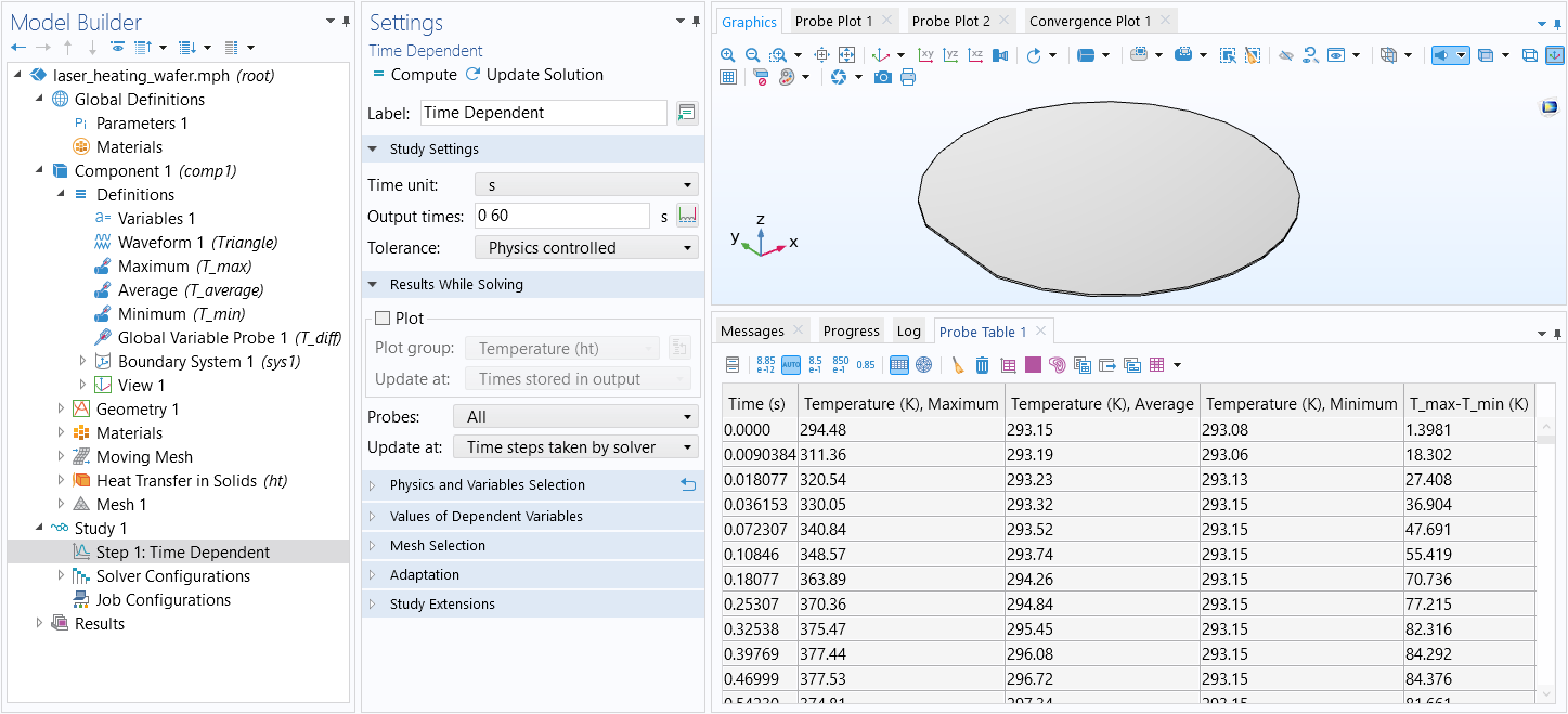 The COMSOL Multiphysics UI showing the Model Builder with the Time Dependent study selected, the corresponding Settings window, the Graphics window showing a silicon wafer model, and the Probe Table.
The probe data table displayed in a tab in the Messages/Progress/Log window. Shown in the Graphics window is the Laser Heating of a Silicon Wafer tutorial model.
After computing the model, the probe data is available under the Results node in the Probe Table node.
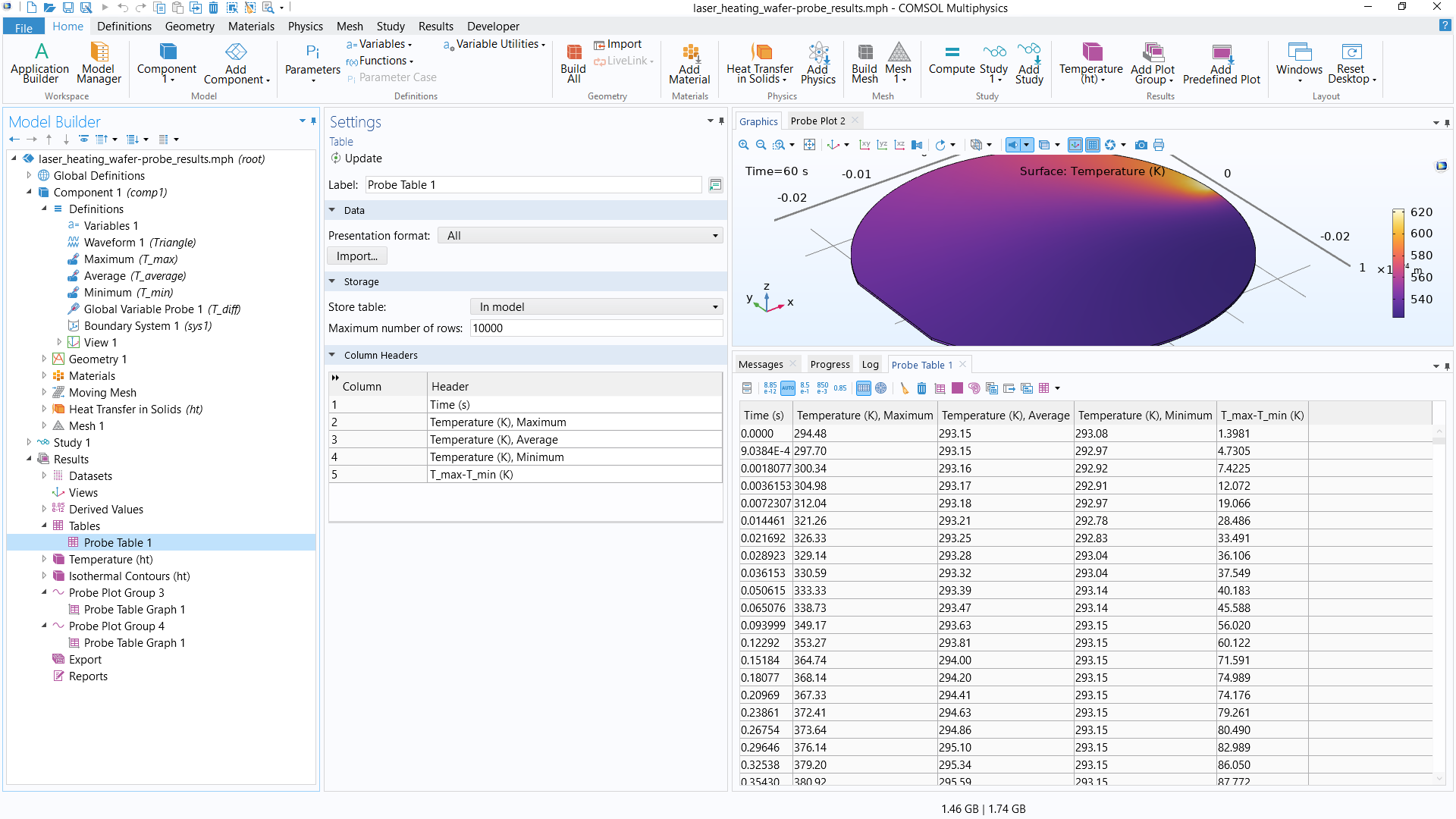 The COMSOL Multiphysics UI showing the Model Builder with the Table node selected, the corresponding Settings window, the Graphics window showing the surface temperature of the silicon wafer model, and the Probe Table.
The Table node containing the probe data from the simulation.
To see another example of using probes, see our blog post "Probing Your Simulation Results".
Using Selections to Reduce the Data Saved
In some instances, you may only be interested in the results in a subset of your model. In cases such as these, you can use geometry selections. You can define one or more selections over geometric entities like domains, boundaries, edges, or points and have the software only store data from those selections. This is done under the Values of Dependent Variables section via the Store fields in output setting.
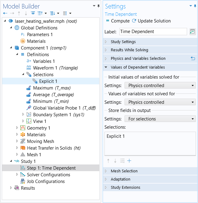
The Store fields in output setting. Here, it is set to only store data from the geometric entities included in the Explicit 1 selection.
When using this option, only the data within one mesh element of the selections will be saved. For a detailed demonstration of this and another technique for reducing the solution data in your model, see our blog post on minimizing your model file size with storing solution techniques.
Removing Parts of the Computed Solutions
Now, say that you already computed a solution but want to remove some parts of it. (One reason for this could be because you need to reduce the size in order to archive the model.) In cases like this, you can use the Combine Solutions study step to remove parts of an existing solution.
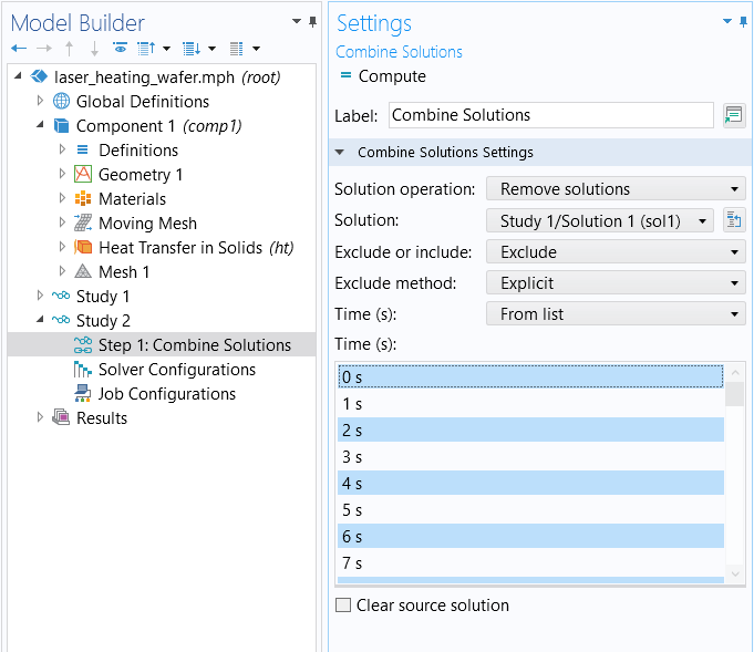
The Combine Solutions study step and it's settings.
To remove parts of an existing solution, you can add a second Empty Study to your model, and under it add a Combine Solutions feature. Then, set the Solution operation to Remove solutions and choose the Solution from which you want to remove stored data. From there, you can either explicitly (pictured in the above screenshot) or implicitly (pictured in the below screenshot) remove or save data from the model.
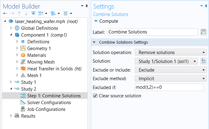
The Implicit option allows an expression to be used to decide which data to keep or remove. The source solution can also be cleared.
You also have the option to completely remove the data from the original study by selecting the Clear source solution option.
Prevent Saving Built, Computed, and Plotted Data
When saving large models, including the computed data can cause the file size to become significantly larger. There are Save options in the root node that enable you to prevent saving built, computed, and plotted data in your model, which can help to reduce the file size.
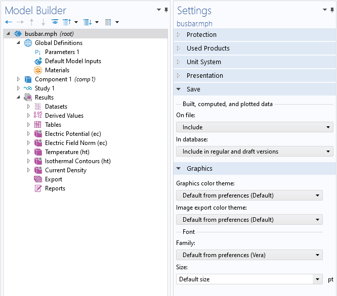
The Save and Graphics sections of the Settings window for the root node.
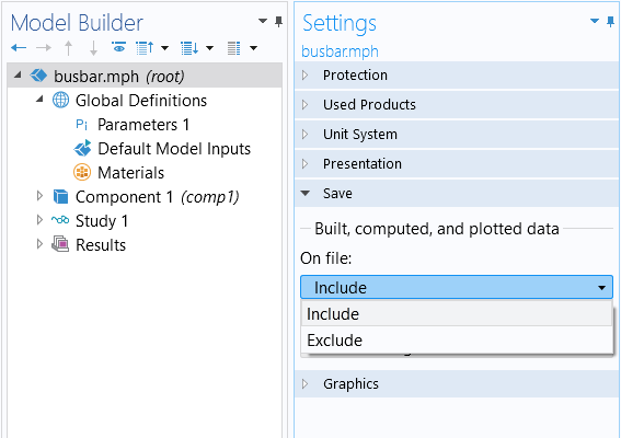 The Model Builder with the root node selected and the Settings window showing the Include and Exclude options for the Built, computed, and plotted data feature.
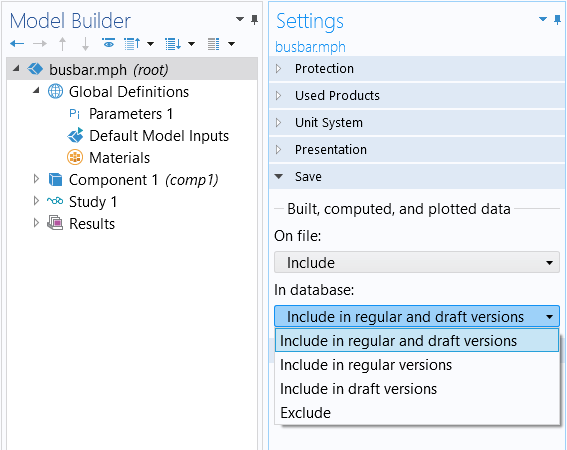 The Model Builder with the root node selected and the Settings window showing the different options for storing a model in a database.
This enables you to reduce the size of a model's MPH-file, as well as reduce the size of a model when it is stored in a database. This functionality is further detailed in the Release Highlights for COMSOL Multiphysics® version 6.0.
Reducing the Size of an Unsolved Model
Even when your model does not contain any results, it can still get quite large. There are several options for reducing the size of a model that has not been computed, such as:
- Saving model files in a compressed state
- Clearing the mesh data
- Clearing the solution data
For instructions on how to implement any of these resolutions, see our Learning Center article on reducing the size of your COMSOL Multiphysics® file.
このページに関するフィードバックを送信, または サポートに連絡 してください.