Problem Description
How, and why, switch between a fully coupled and a segregated approach to solving a multiphysics model?
How, and why, switch between the direct and iterative linear system solver?
Solution
Fully Coupled versus Segregated solution approach
When solving a multiphysics model, there are two approaches that can be taken to solving the (usually nonlinear) system of equations that describe the solution.
The Fully Coupled approach forms a single large system of equations that solve for all of the unknowns (the fields) and includes all of the couplings between the unknowns (the multiphysics effects) at once, within a single iteration.
On the other hand, the Segregated approach will not solve for all of the unknowns at one time. Instead, it subdivides the problem up into two or more Segregated Steps. Each step will usually represent a single physics, but sometimes even a single physics can be subdivided into steps, and sometimes one step can contain multiple physics. These individual segregated steps are smaller than the full system of equations that are formed with the Fully Coupled approach. The Segregated steps are solved sequentially within a single iteration, and thus less memory is required.
The software will automatically select the segregated approach in many cases, especially 3D models. On the other hand, the fully coupled approach is used by default for most 2D models. These default settings are chosen for general robustness.
Regardless of the approach to solving nonlinear problems, the solution is approached by iteration. That is, the Fully Coupled or Segregated approach is called repeatedly, and gradually converges to the solution of the nonlinear problem. Since the Fully Coupled approach includes all coupling terms between the unknowns, it often converges more robustly and in less iterations as compared to the Segregated approach. However, each iteration will require relatively more memory and time to solve, so the Segregated approach can be faster overall. For general guidance in solving nonlinear models, see: Knowledge Base 103: Improving Convergence of Nonlinear Stationary Models . For guidance on how to reduce memory requirements, see Knowledge Base 1030: Error: "Out of memory".
Setting up the Fully Coupled or Segregated approach
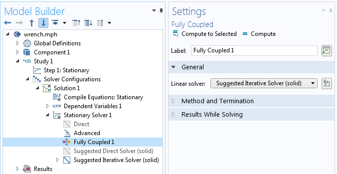
To use the Fully Coupled approach in a model that is currently using the Segregated approach, expand out the Study > Solver Configurations settings and look for either the Stationary Solver or the Time-Dependent Solver feature. Right-click on this feature and select Fully Coupled and a new Fully Coupled feature will appear in the solver sequence, and the Segregated Solver will become greyed out.
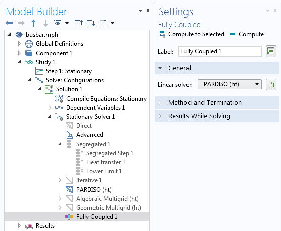
The Fully Coupled feature.
To set up the Segregated approach, right-click on the Stationary Solver or the Time-Dependent Solver feature and select Segregated to add a new Segregated feature. Then, right-click on the Segregated feature and add at least two Segregated Steps and select the variables that correspond to the physics that you want to solve within that step.
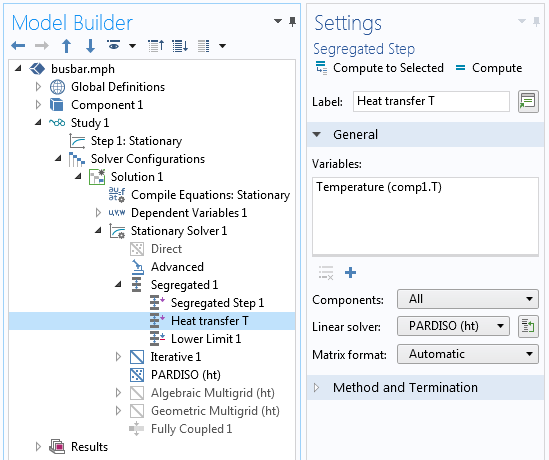
The Segregated feature and the Segregated Step subfeature.
Direct versus Iterative Linear System Solvers
Regardless of the full coupled or segregated approach, within each iteration a linearized system of equations is solved. There are two classes of algorithms available for solving linear systems of equations, the Direct and the Iterative solvers.
Direct solvers have the advantage of being the most robust and general. They have the drawback of requiring relatively a lot of memory and time, and memory requirements and solution time go up rapidly with increasing problem size. Iterative solvers require less memory and time, and these scale more slowly with increasing model size. However, iterative solvers are less robust, their convergence will be slower for so-called ill-conditioned problems. Ill-conditioned problems can arise when, for example, there is a very high contrast in material properties, or the geometric aspect ratio is very high. Examples of problems that are nearly ill-conditioned include the structural bending of a very long slender beam or an electric currents model where the material electric conductivity is different by several orders of magnitude.
The Direct solvers available within COMSOL Multiphysics are PARDISO, MUMPS, and SPOOLES, as well as a Dense Matrix Solver. Either PARDISO or MUMPS are likely the fastest, and SPOOLES will likely use the least memory. All should converge to the same answer. The Dense Matrix Solver should only be used for Boundary Element Method models.
There are many different types of Iterative solvers available and each contains several lower-level settings. Manually choosing an iterative solver and adjusting these settings is not usually advised. When an appropriate iterative solver is known for a particular problem, the software will automatically present that combination as an option.
Also be aware that as you perform a Mesh Refinement Study (see: Knowledge Base 1261: Performing a Mesh Refinement Study ) the software may automatically switch between direct and iterative solvers, as governed by the number of degrees of freedom. If you've manually changed solver settings, you may need to manually switch to an iterative solver for larger problems, if it makes sense to do so.
Selecting a Direct or Iterative Solver
To switch between the Direct or Iterative linear system solver, go to either the Fully Coupled feature (if a Fully Coupled approach is being used) or one of the Segregated Step features (if the Segregated approach is being used) and, within the General section, change the Linear Solver to one of the available options.
The iterative solver being used within the Fully Coupled feature.
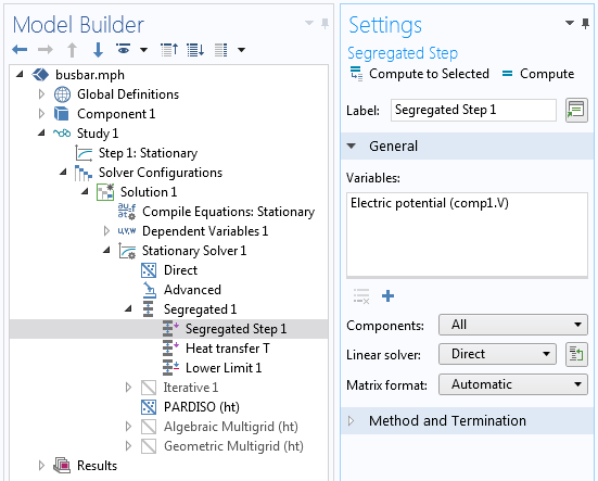
The direct solver being used within a Segregated Step feature.
COMSOL は, 本ページに掲載されている情報の確認に合理的な努力を払っております. リソースおよびドキュメントは情報提供のみを目的としており, COMSOL はその有効性について明示的または黙示的な保証を行いません. 開示されたデータの正確性について, COMSOL は法的責任を負いません. 本文書で言及されている商標はすべて, それぞれの所有者に帰属します. 商標に関する詳細は, 製品マニュアルをご参照ください.