

The last two blog posts in the Chemical Kinetics series were concerned with modeling chemical reactions based on a particular set of parameters. While this is important and of great academic and industrial interest, the relevant parameters were assumed. Now, let’s find out how to estimate the chemical parameters using COMSOL Multiphysics.
Chemical Parameters
To quote a favorite phrase of my former professor: “A good and benevolent fairy waved her wand and gave us the activation energy.” The truth is, these parameters (rate constant, activation energy, and pre-exponential factor) are the result of a great number of repeated experiments. Almost all of the experimental laboratory work I did during my research career involved running chemical reactions at different temperatures, sampling at regular intervals, transforming the results, and calculating rate constants.
Diazo Compounds, Dangerously Explosive
Have a look at the structure of the chemical compound benzenediazonium chloride (BDC):

As innocuous as that little structure seems, it packs a punch. It belongs to the family of the diazo compounds (meaning with a carbon atom, C, adjacent to two connected nitrogen, N, atoms) a group of compounds that are dangerously explosive.
When Does BDC Decompose?
Recall from this series’ first blog entry on the Arrhenius Law that any molecule requires a particular amount of energy to overcome its inherent “laziness” or resistance to reaction — this reaction is the activation energy. Today, I will describe how a careful series of experiments (along with some calculations in COMSOL Multiphysics) can give you precisely that energy, thus allowing a statement on the safety of a particular process.
The Experiments
The decomposition of BDC proceeds irreversibly (as would be expected from an explosion), so we can write the fairly simple reaction equation:
BDC → Products
This corresponds to the rate equation (again, see “A General Introduction to Chemical Kinetics, Arrhenius Law” for details):
(1)
with the related ordinary differential equation (ODE):
(2)
If we recall the Arrhenius equation
(3)
the problem becomes relatively clear. By performing the decomposition reaction at various temperatures and measuring BDC concentration at different times, we can fit the values of A and E_\mathrm{A} to best reflect the experimental results with the modeled ODE solution.
Of course, the above rate equation can be integrated directly and in practice we would use our knowledge of the concentration vs. time expression (we derived a similar expression in the post on the Arrhenius Law ) to determine the rate constant directly from the gradient of a straight-line plot of \ln{c_\mathrm{BDC}} against t. Then we can plot \ln k against 1/T to find the activation energy, which in practice can be seen as a graphical least square problem since the experimental points will never be “perfectly” aligned.
Here we will use the Parameter Estimation tool to demonstrate the corresponding numerical solution for this simple case. Automated parameter estimation becomes much more valuable when used for chemical mechanisms where we don’t know the expressions for concentration as a function of time in closed form, and so we have to proceed by modeling.
Estimating Chemical Parameters in COMSOL Multiphysics
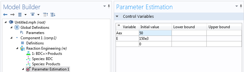
Using the Model Builder, we can select the 0D Reaction Engineering interface with a time-dependent study from the Model Wizard. We input the reaction via BDC → Products and define an initial BDC concentration of 1 mol/L. Defining a parameter called “Tiso” (for the system temperature) and setting the temperature to this parameter is just a matter of three clicks. By right-clicking the Reaction Engineering node we can add a Parameter Estimation interface where we can choose our control variables and define our least square problem.
We can actually reduce the computational effort significantly if we choose not to optimize for A, but rather for eA. This way, the solver is dealing with two exponential dependencies at the same time — rather than one linear and one exponential. Suitable initial values are a matter of experience; both activation energies of around 150 kJ/mol and prefactors of around e50 are reasonable.
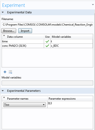
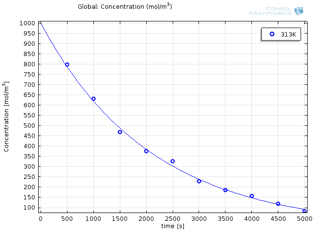
Getting the experimental data into COMSOL Multiphysics® is as easy as right-clicking Parameter Estimation, selecting the option to load from file, and selecting the corresponding .csv-file (these files can be easily exported from Excel®). At the bottom of the Experiment settings window, we can select the experimental parameter that was varied for the experiments. The data is automatically plotted after the import, so we can ensure it makes sense:
Finally, we can select the option to use the Arrhenius expression from the Reaction settings window and type in the control variable names (“exp(Aex)” for the prefactor and “E” for the activation energy). By choosing study times between 0 and 5,000 seconds, we ensure all the experimental data is accounted for.
Getting the Study Right
Choosing a solver in the study depends on the purpose, and the choice is usually done from experience. In the case of parameter estimations for reaction engineering, the Levenberg-Marquardt solver is often the best choice, as it is well established in the field of parameter estimation for reaction kinetics. While running the simulation only takes a few seconds, the results are striking:
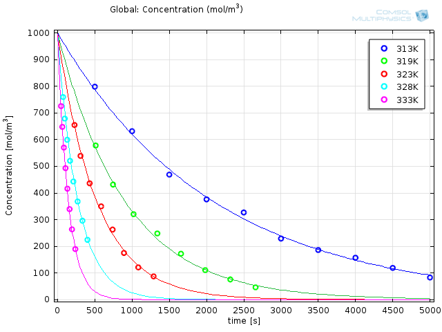
Modeled results with optimized reaction parameters (solid lines) together with experimental results (o).
The obtained values are e36.9s-1 and 116 kJ/mol for the prefactor and the energy, respectively. Experimental work is tricky at best; it requires patience, precision, and a great deal of nerve. By making the import and interpretation of your experimental data this easy, you can focus on what’s really important.
Next Up
The next blog post in this Chemical Kinetics series will look at another way of getting external data into your system — by using interpolation functions for thermodynamics. In doing so, we will come across one of the most fascinating processes in industrial chemistry. A reaction with a history as dramatic and complex as Tolstoy’s War and Peace! Stay tuned.


Comments (2)
Jahid Ferdous
October 30, 2014Hi,
i am very new in comsol optimization. I am just wondering whether you have any model for this example by any chance.
Thanks in advance.
Jahid
Eyal Spier
October 31, 2014Dear Jahid,
Thank you very much for your comment.
If you have access to the Chemical Reaction Engineering and Optimization Modules, you can find the model in your model library. Just go to “File”, “Model Libraries” and search for the model “Activation Energy”.
All the best,
Eyal