アプリケーションギャラリには電気, 構造, 音響, 流体, 熱および化学分野に関連する COMSOL Multiphysics® チュートリアルおよびデモアプリファイルが用意されています. これらの例はチュートリアルモデルまたはデモアプリファイルとそれに付随する手順をダウンロードすることにより独自のシミュレーション作業の開始点として使用できます.
クイック検索機能を使用して専門分野に関連するチュートリアルやアプリを検索します. MPHファイルをダウンロードするには, ログインするか, 有効な COMSOL ライセンスに関連付けられている COMSOL Access アカウントを作成します. ここで取り上げた例の多くは COMSOL Multiphysics® ソフトウェアに組み込まれ ファイルメニューから利用できるアプリケーションライブラリからもアクセスできることに注意してください.

This example models the desalination of water by capacitive deionization in a "flow-between" cell (fbCDI). The model geometry is in 2D. Steady Brinkman flow, a tertiary current distribution, and the improved modified Donnan description of the deionization process is assumed. 詳細を見る
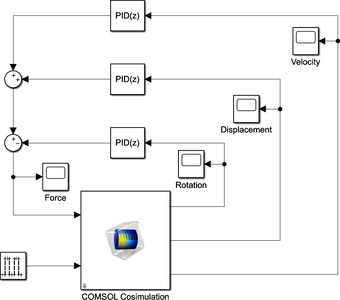
This model shows how to control the position of the base of an inverted pendulum to keep it vertical. The control is performed using a PID controller in Simulink®. The position of the base is constrained within specified limits, and an external force is applied at the base to keep it ... 詳細を見る

The present example simulates the turbulent flow over a 3D hill geometry using the Large Eddy Simulation (LES) interface with synthetic turbulence at the inlet boundary. 詳細を見る

This model computes the fundamental eigenfrequency and eigenmode for a tuning fork that is synchronized from SOLIDWORKS® via the LiveLink™ interface. The length of the fork is then optimized so that the tuning fork sounds the note A, 440 Hz. 詳細を見る

This model computes the fundamental eigenfrequency and eigenmode for a tuning fork that is synchronized from Solid Edge® via the LiveLink™ interface. The length of the fork is then optimized so that the tuning fork sounds the note A, 440 Hz. 詳細を見る

This model computes the fundamental eigenfrequency and eigenmode for a tuning fork that is synchronized from PTC Creo Parametric™ via the LiveLink™ interface. The length of the fork is then optimized so that the tuning fork sounds the note A, 440 Hz. 詳細を見る
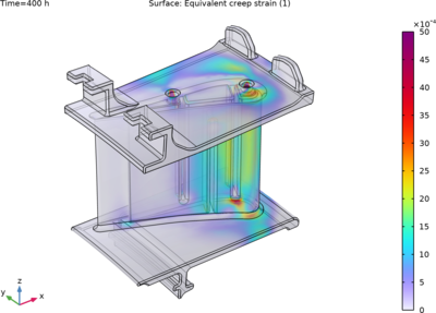
This example shows how to compute deformations caused by secondary creep in a turbine stator blade. The creep rate is highly influenced by temperature, and the deformation and stress relaxation is thus controlled by the temperature field. 詳細を見る

In this example, phase transformation data and phase material properties are imported from JMatPro, and used to compute CCT curves. Dilatometry curves (axial thermal strain) are computed across a range of cooling rates. 詳細を見る

This tutorial model shows the setup of a 2D axisymmetric stress analysis, through contact, of a 3D threaded pipe fitting. The example involves synchronizing the 3D Solid Edge® geometry and selections, which specify the faces in contact, with the 2D geometry in COMSOL ... 詳細を見る

This tutorial model shows the setup of a 2D axisymmetric stress analysis, through contact, of a 3D threaded pipe fitting. The example involves synchronizing the 3D Inventor® geometry and selections, which specify the faces in contact, with the 2D geometry in COMSOL Multiphysics ... 詳細を見る