有限要素解析 (FEA) ソフトウェア
What Does Finite Element Analysis Software Bring?
The purpose of finite element analysis (FEA) software is to reduce the number of prototypes and experiments that have to be run when designing, optimizing, or controlling a device or process. This does not necessarily mean that companies and research institutes save money by adopting FEA. They do, however, get more development for their dollar, which may result in gaining a competitive edge against the competition. For this reason, it may be reasonable to increase research and development resources for FEA.
Once an FEA model is established and has been found useful in predicting real-life properties, it may generate the understanding and intuition to significantly improve a design and operation of a device or process. At this stage, optimization methods and automatic control may provide the last degree of improvements that can be difficult to obtain with intuition only. Most modern FEA software features methods for describing automatic control and incorporating such descriptions in mathematical and numerical models. Optimization methods are usually included in the solution process, which is further described in detail below.
The introduction of high-fidelity models have also contributed to an accelerated understanding. This has sparked new ideas and completely new designs and operation schemes that would have been hidden or otherwise impossible without modeling. Therefore, FEA is an integral tool for research and development departments in companies and institutions that operate in highly competitive markets. Over time, the use of FEA software has expanded from larger companies and institutions that support educating engineers to smaller companies in many different industries and institutions with a wide variety of disciplines.
Inside FEA Software
The foundation of FEA software is formed by the laws of physics expressed in mathematical models. In the case of FEA, these laws consist of different conservation laws, laws of classical mechanics, and laws of electromagnetism.
The mathematical models are discretized by the Finite Element Method (FEM), resulting in corresponding numerical models. The discretized equations are solved and the results are analyzed, hence the term finite element analysis.
The language of mathematics is required to describe the laws of physics, which – for space and time-dependent descriptions – result in partial differential equations (PDEs). The solution to the PDEs is represented by dependent variables, such as structural displacements, velocity fields, temperature fields, and electric potential fields. The solution is described in space and time, along the independent variables x, y, z, and t.
The purpose of these descriptions is found in the study of the solution to the PDEs for a given system, which results in understanding a studied system and the ability to make predictions about it. FEA is used to understand, predict, optimize, and control the design or operation of a device or process.
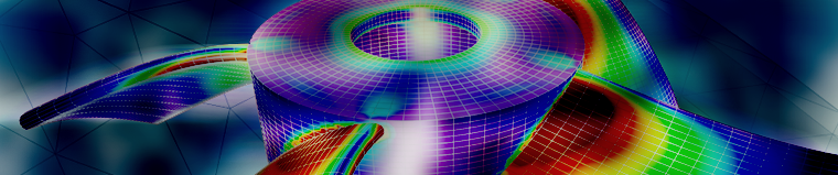
 Cooling fan blade vibration, which was predicted by structural mechanics mode shape analysis.
Cooling fan blade vibration, which was predicted by structural mechanics mode shape analysis.
Cooling fan blade vibration, which was predicted by structural mechanics mode shape analysis.
For structural mechanics, the physical descriptions are based on the laws for the balance of forces and the constitutive relations that relate the stresses to strains. An example of such a constitutive relation is Hooke’s law. Traditional FEA often refers to structural analysis only.
 A CFD simulation example.
A CFD simulation example.
A CFD simulation example.
In fluid flow, heat transfer, and mass transfer, the descriptions are based on the laws for conservation of momentum, mass, and energy. The fluxes in these conservation laws are typically composed of advection and dissipation or diffusion. The precise form of the dissipation and diffusion is given by a constitutive relation, such as the viscous stress for Newtonian fluids, Fourier’s law of thermal conduction, and Fick’s law of diffusion.
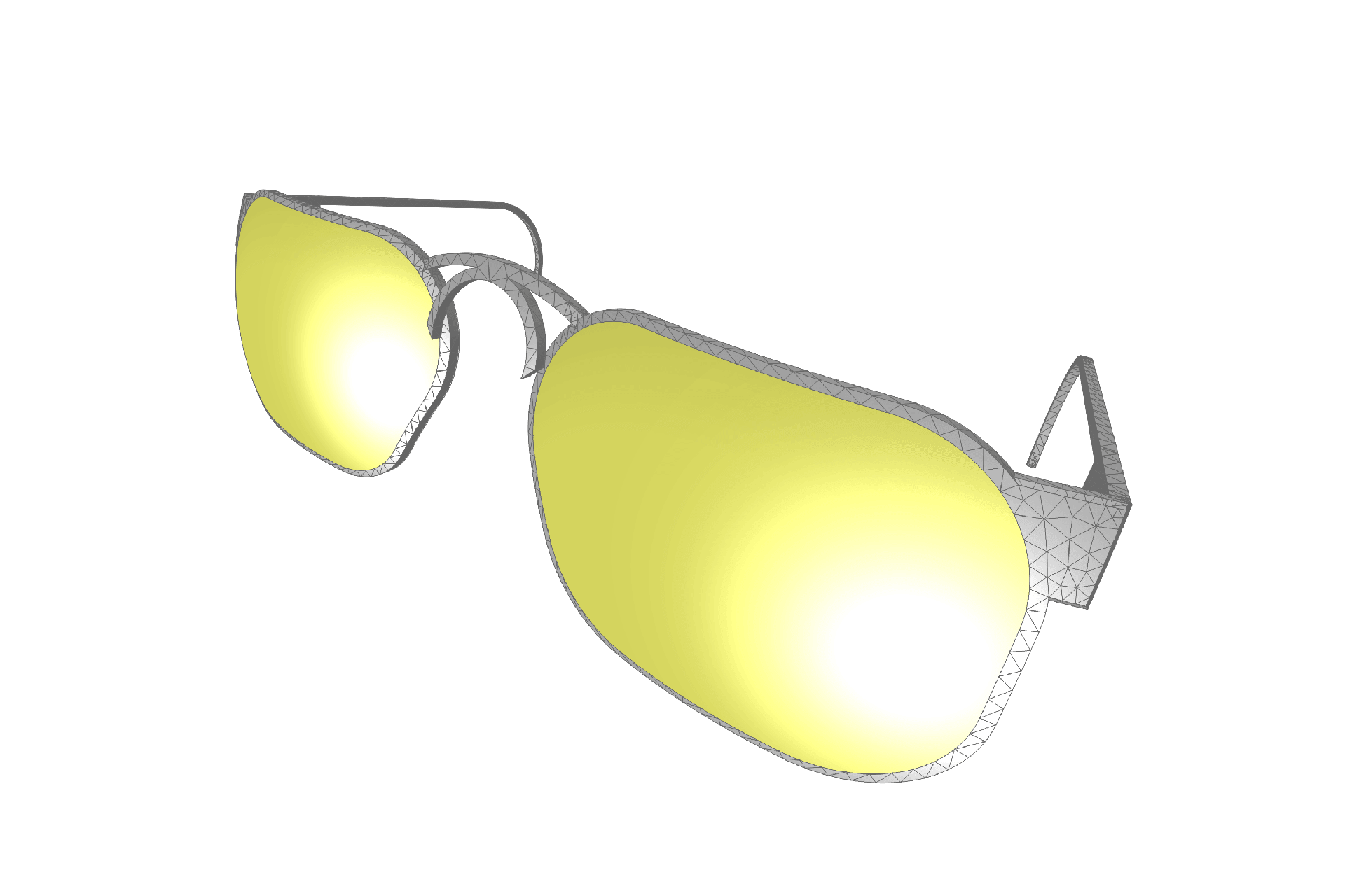
 Radiation diagram around the GPS frequency range of a probe-fed corner-truncated microstrip patch antenna. The arrows show the right-hand circular polarization with almost radial components. The near spherical surface indicates the magnitude of gain.
Radiation diagram around the GPS frequency range of a probe-fed corner-truncated microstrip patch antenna. The arrows show the right-hand circular polarization with almost radial components. The near spherical surface indicates the magnitude of gain.
Radiation diagram around the GPS frequency range of a probe-fed corner-truncated microstrip patch antenna. The arrows show the right-hand circular polarization with almost radial components. The near spherical surface indicates the magnitude of gain.
A static electric field is related to the amount of electric charge through the Gauss law and the magnetic field to electrical currents by Ampere's law. Maxwell's equations bring dynamics, such as the induction of an electric field from a time-varying magnetic field, by Faraday's law. Maxwell's own decisive contribution was the addition of the displacement current from a time-varying electric field, which completed the description of the wave nature of electromagnetic fields.
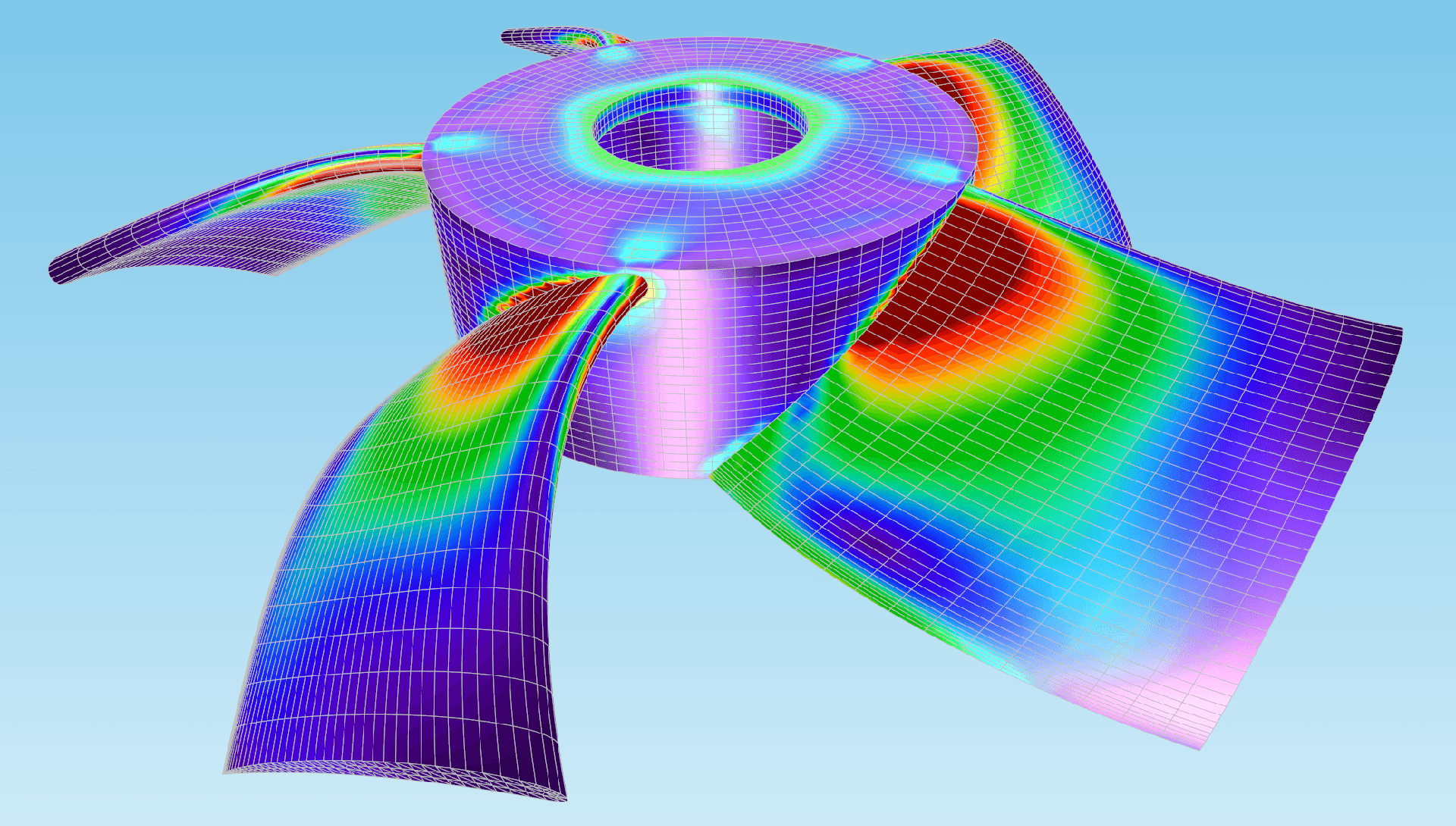
A MEMS actuator uses the joule heating effect to create thermal expansion of the two hot arms (white and yellow colors) that carry an electric current. The thermal expansion creates a structural displacement that moves the actuator. This is a typical case of multiphysics in FEA. You can follow this model being built from scratch in the following video: How to Set Up and Run a Simulation with COMSOL Multiphysics.
A MEMS actuator uses the joule heating effect to create thermal expansion of the two hot arms (white and yellow colors) that carry an electric current. The thermal expansion creates a structural displacement that moves the actuator. This is a typical case of multiphysics in FEA. You can follow this model being built from scratch in the following video: How to Set Up and Run a Simulation with COMSOL Multiphysics.
The laws used in structural mechanics, fluid flow, heat transfer, mass transfer, and electromagnetism can be combined to describe systems where several phenomena interact, which is usually referred to as multiphysics systems. For example, the description of microelectromechanical systems (MEMS) usually requires combining the laws of structural mechanics and electromagnetism. The description of fluid-structure interaction (FSI) requires the combination of the laws of structural mechanics and fluid flow.
Mathematical Model and Numerical Model
A mathematical model of a system can consist of one or several PDEs that describe the relevant laws together with boundary and initial conditions. The boundary conditions impose extra conditions on the solution and on a part of the modeled domain (e.g., surfaces, edges, or points). Several different boundary conditions can be used for the same model. The initial conditions define the state of the system in the beginning of a time-varying event.
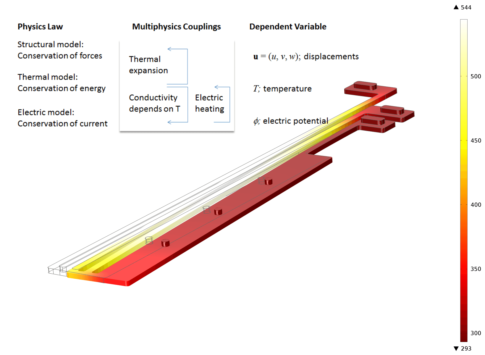
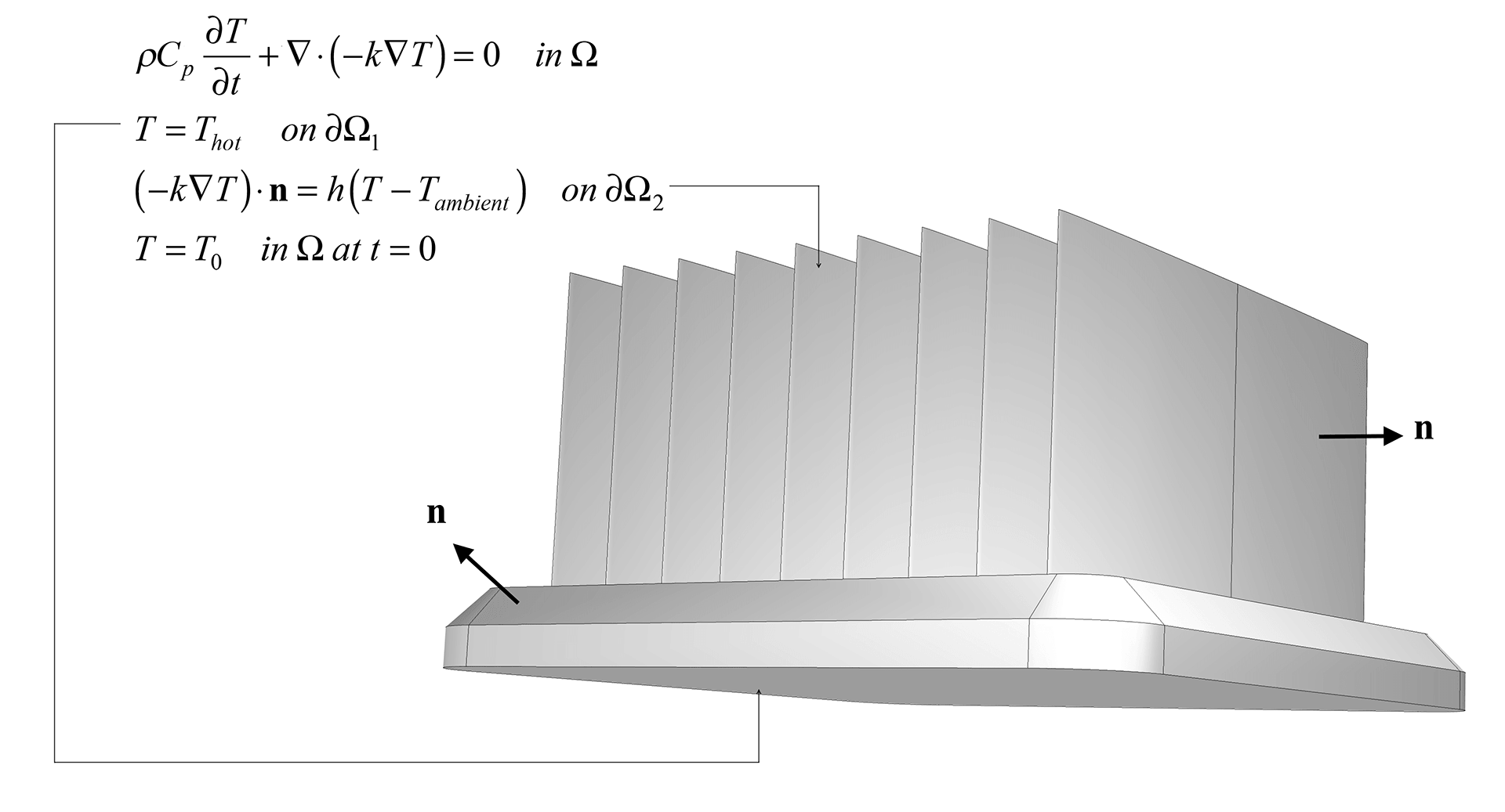 A mathematical model of a heat sink is based on the conservation of energy yielding the heat equation for the temperature field, T, which is the first equation in the figure above. The constitutive relation is Fourier's law for heat conduction, where k denotes the thermal conductivity. The equation above is valid inside the heat sink domain (Ω), where ρ denotes the density of the material and Cp, the heat capacity. At the base of the heat sink (∂Ω1), the temperature, denoted as T, is constrained to Thot in the second equation above, which represents the first boundary condition. At all other boundaries (∂Ω2), except for the base, the heat flux at every point on this boundary is proportional to the temperature jump to the ambient temperature just outside the boundary layer. h denotes the heat transfer coefficient and n, the outwards pointing normal vector, of length unity, to the boundary surface. If the ambient temperature is lower than the local heat sink temperature, then heat leaves the heat sink.
A mathematical model of a heat sink is based on the conservation of energy yielding the heat equation for the temperature field, T, which is the first equation in the figure above. The constitutive relation is Fourier's law for heat conduction, where k denotes the thermal conductivity. The equation above is valid inside the heat sink domain (Ω), where ρ denotes the density of the material and Cp, the heat capacity. At the base of the heat sink (∂Ω1), the temperature, denoted as T, is constrained to Thot in the second equation above, which represents the first boundary condition. At all other boundaries (∂Ω2), except for the base, the heat flux at every point on this boundary is proportional to the temperature jump to the ambient temperature just outside the boundary layer. h denotes the heat transfer coefficient and n, the outwards pointing normal vector, of length unity, to the boundary surface. If the ambient temperature is lower than the local heat sink temperature, then heat leaves the heat sink.
A mathematical model of a heat sink is based on the conservation of energy yielding the heat equation for the temperature field, T, which is the first equation in the figure above. The constitutive relation is Fourier's law for heat conduction, where k denotes the thermal conductivity. The equation above is valid inside the heat sink domain (Ω), where ρ denotes the density of the material and Cp, the heat capacity. At the base of the heat sink (∂Ω1), the temperature, denoted as T, is constrained to Thot in the second equation above, which represents the first boundary condition. At all other boundaries (∂Ω2), except for the base, the heat flux at every point on this boundary is proportional to the temperature jump to the ambient temperature just outside the boundary layer. h denotes the heat transfer coefficient and n, the outwards pointing normal vector, of length unity, to the boundary surface. If the ambient temperature is lower than the local heat sink temperature, then heat leaves the heat sink.
From a physical point of view, the boundary conditions and the initial data are often a natural part of the model (e.g., loads and constraints for structural mechanics, pressure levels at inlets and outlets for fluid flow, and the electric potential for terminals in electrostatics). From a mathematical point of view, the boundary conditions and the initial data are what singles out a unique solution among the infinitely many alternatives.
Well-Posed Mathematical Models
If a mathematical model is properly defined, it may also be well posed. A mathematical model is well posed if it has a unique solution that continuously depends on the problem data (i.e., source terms, fluxes, constraint values, and initial values). If the model is not well posed, this will be reflected in the numerical model and will cause problems in the solution process.
Being well posed can be seen as the model's minimal requirement to be used for numerical simulations, such as in FEA.
From a theoretical point of view, it is usually very difficult to determine if a realistic nonlinear 3D model is well posed or not and, for this reason, greatly simplified models are instead used in fundamental analysis. The conclusions drawn from these simplified models are used to estimate how more realistic models behave. Even a well-posed model can be very sensitive to changes in the model data. Such models are inherently ill-conditioned or sensitive.
Modern numerical methods for solving PDEs have revolutionized applied mathematics. The reason is that analytical solutions to mathematical models can only be found in very special cases, such as in certain combinations of equations and simple geometries. While these cases are important from a theoretical point of view, they are often of little use to the engineer. Numerical methods do not have this limitation, so they can handle nonlinear problems as well as complicated geometries. Other computational challenges exist for numerical methods (see the "Solution" section below), but the applicability to new models and geometries is not one of them.
Numerical methods are able to give an approximation of the solution to a well-posed mathematical model. Most numerical methods are based on a discretization of the modeled domain and the described dependent variables. The finite difference, volume, and element methods are the most commonly used methods for this discretization. As the name reveals, the finite element method (FEM) is used in finite element analysis.
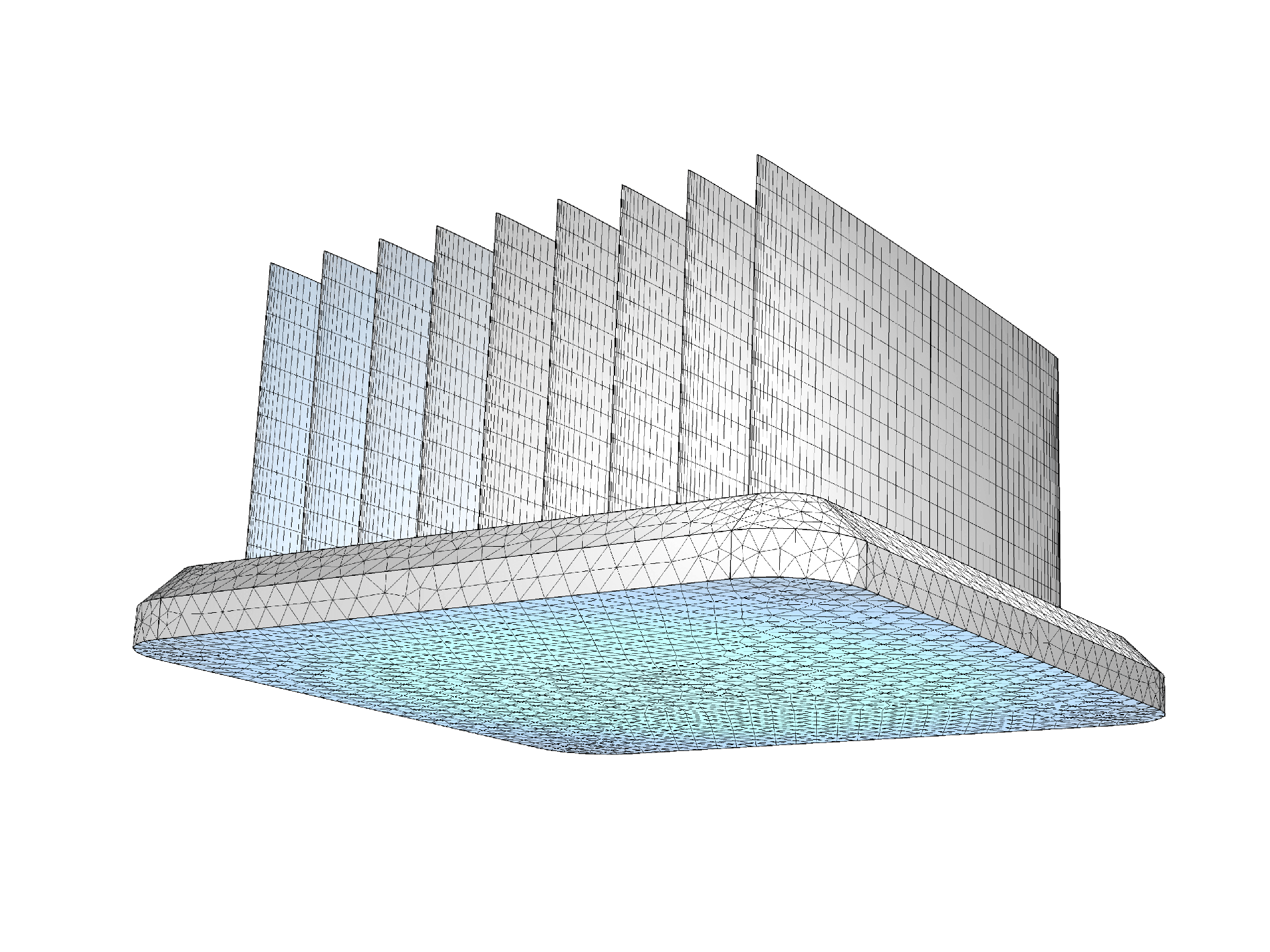 The heat sink model discretized by finite elements. The tetrahedral finite element volume mesh in the base gives triangular surface elements. The prism elements in the fins give rectangular elements on the fin surfaces.
The heat sink model discretized by finite elements. The tetrahedral finite element volume mesh in the base gives triangular surface elements. The prism elements in the fins give rectangular elements on the fin surfaces.
The heat sink model discretized by finite elements. The tetrahedral finite element volume mesh in the base gives triangular surface elements. The prism elements in the fins give rectangular elements on the fin surfaces.
The discretization of a mathematical model results in a numerical model for the described system, where the numerical model is a discrete approximation of the mathematical model. The error introduced by using the numerical model instead of the mathematical model is referred to as the truncation error.
The truncation error is defined as the difference between the solution to the numerical and mathematical model. If the numerical model is stable and consistent, then the truncation error approaches zero, as the element sizes approach zero (i.e., the numerical solutions converge to the solution to the mathematical model). The truncation error then converges at a certain rate, measured by the order of accuracy. Consistency is equivalent to a positive order of accuracy.
The starting point of the finite element method is the weak formulation of the mathematical model. This form can be obtained from the pointwise PDEs (also called the strong form) by introducing test functions, multiplying the PDEs with these test functions, and then integrating them over the modeled domain. This procedure can be optionally combined with integration by parts. For each test function, the integral relation must hold. To be consistent with the PDEs, there must be infinitely many test functions that must be general enough. Therefore, infinitely many integral relations must hold, whereas the pointwise PDEs must hold for each point in the modeled domain.
The finite element method introduces test functions that are defined through a computational mesh. For each computational cell, or mesh element, a number of test functions are locally defined. Additionally, as part of the finite element method, shape functions are defined. These are used to represent the candidate solution. For time-dependent problems, the finite element method is often only used for the spatial discretization. In this case, the system of equations, obtained after the finite element discretization, is a system of ordinary differential equations (ODEs). This system may, in turn, be discretized with a finite difference method or other similar methods.
In the example here, the approximation for the temperature is written as:
(1)

where  denotes the shape functions and
  denotes the unknown weights.
Here, the shape functions vary only in space, while the unknowns vary only in time. The weights are also called the degrees of freedom in a finite element method. In the Galerkin finite element method, the shape functions are of the same sort as the test functions. The weak form, together with the boundary conditions, is then used to formulate a finite algebraic system of equations for the unknowns.
Each node in the mesh, denoted j, has a basis or test function, , and gives an equation according to the following:
(2)

For every node j, there are only a few shape functions i that overlap with the test function j, so the integrals above have to be evaluated only over elements that share the same node j. Note that the boundary contribution is nonzero if node j is a boundary node. This is a linear ordinary differential equation for the unknowns, at least if the material properties do not depend on the temperature.
This is a general rule of thumb: If the system of PDEs is nonlinear, then the problem for the unknowns is also nonlinear. Also note that only the flux boundary condition is included in this system of equations. The condition of prescribed temperature is not included and has to be added as extra constraints.
The finite element method gives considerable freedom in selecting test and shape functions for different mesh element types and equations. The finite element formulation on "unstructured" meshes, where the size and aspect of the participating elements can differ greatly, makes the method applicable for very complex geometries at a relatively low cost. Unstructured meshes are also relatively easy to automatically produce. In most cases, the shape and test functions are low-order polynomials that are easy to define and integrate. Furthermore, the close relationship with the weak form gives the method a thorough mathematical ground, where the mathematical theory is very well developed.
Once the mathematical model has been discretized, the equations in the resulting numerical model have to be solved.
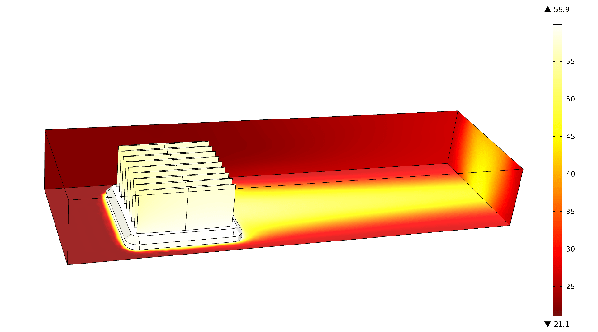 The temperature in the heat sink varies only to a small degree, compared to the temperature in the surrounding air that flows from left to right. The small variation is expected, since the heat sink material (aluminum) has a much higher thermal conductivity than air, which is also poorly mixed. In this simulation, the heat sink model is expanded with the equations for conservation of energy in the air around the heat sink and the fluid flow equations, which express conservation of mass and momentum. The whole system of equations is discretized and solved with the finite element method.
The temperature in the heat sink varies only to a small degree, compared to the temperature in the surrounding air that flows from left to right. The small variation is expected, since the heat sink material (aluminum) has a much higher thermal conductivity than air, which is also poorly mixed. In this simulation, the heat sink model is expanded with the equations for conservation of energy in the air around the heat sink and the fluid flow equations, which express conservation of mass and momentum. The whole system of equations is discretized and solved with the finite element method.
The temperature in the heat sink varies only to a small degree, compared to the temperature in the surrounding air that flows from left to right. The small variation is expected, since the heat sink material (aluminum) has a much higher thermal conductivity than air, which is also poorly mixed. In this simulation, the heat sink model is expanded with the equations for conservation of energy in the air around the heat sink and the fluid flow equations, which express conservation of mass and momentum. The whole system of equations is discretized and solved with the finite element method.
The Processes Involved in Finite Element Analysis
For historical reasons, traditional finite element analysis refers to models based around structural mechanics and, to a lesser extent, heat transfer. Since the popularity of modeling multiphysics applications has increased, and due to the fact that the finite element method is widely used for fluid flow and electromagnetics simulations, the term “finite element analysis” has also become more accepted in other engineering and science fields. No matter what the application field is, the processes involved in finite element analysis are the same.
Below is a summary of the main workflow, from geometry to model documentation.
Geometry
Finite element analysis requires that the model geometry is “water tight”. Computer aided design (CAD) geometries are not always used for analysis. This implies that, for example, something that is a volume in the real world can be described by a set of loosely connected 3D surfaces in a CAD drawing. In finite element analysis, these surfaces have to actually form a real volume.
Even if a set of 3D surfaces in a CAD drawing do form a volume, some surfaces may be slender and some edges may be unnecessarily short in relation to the size of the geometry. This results in an undesirable concentration of elements at the offending geometrical features.
In order to prepare a CAD geometry for finite element analysis, repairing and defeaturing of the geometry is often required. Repairing patches the parts of the geometry that are not “water tight”, while defeaturing may remove slender surfaces or merge unnecessary small edges.
The process of creating, repairing, and defeaturing CAD geometry for analysis is usually part of a larger process traditionally denoted as preprocessing in FEA.
Materials
The constitutive laws in a mathematical model involve physical properties of the materials. The properties may depend on the modeled variables (the "dependent variables"). For example, in an analysis of thermal expansion, mechanical and thermal properties often depend on the temperature.
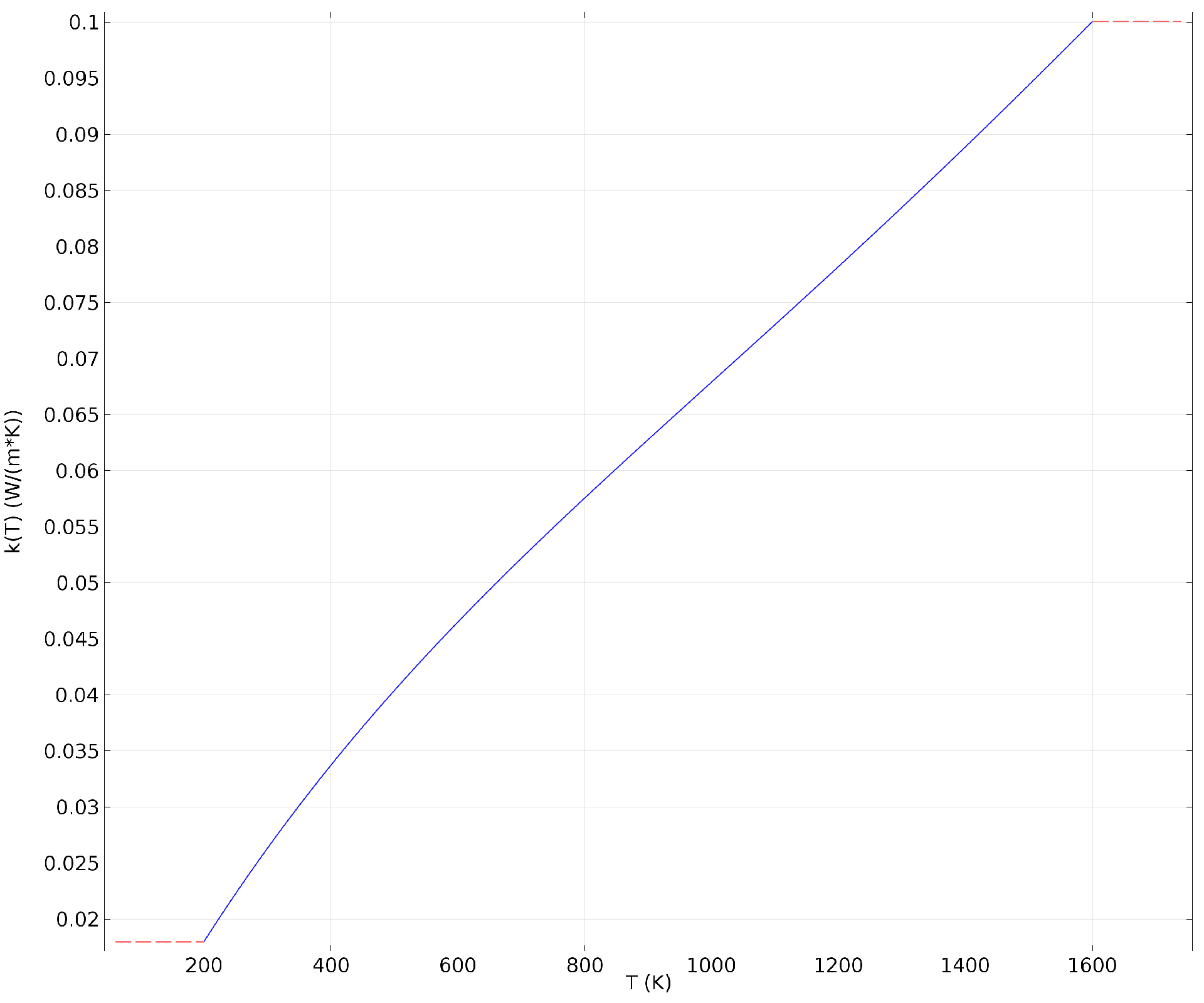 Thermal conductivity of air as a function of temperature.
Thermal conductivity of air as a function of temperature.
Thermal conductivity of air as a function of temperature.
In practice, this involves estimating the correct validity intervals for the material properties and the correct reference point. In addition, different materials have to be attributed to the different parts of the geometry.
In traditional FEA, the process of defining and attributing material properties and functions of the material properties is usually also regarded as being a part of preprocessing.
Domain Settings, Boundary Conditions, Loads, and Constraints
In structural mechanics, the mathematical model may be defined by the selected materials, loads, and constraints on the system. In general, the materials, domain equations, boundary conditions, and initial conditions define the mathematical model.
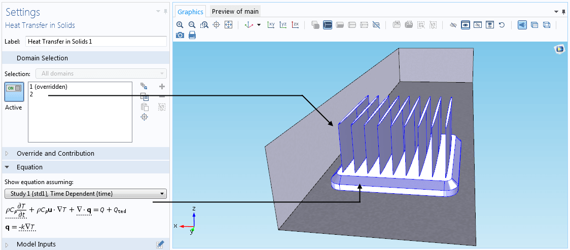 The domain equations in the heat sink are automatically defined by selecting the Heat Transfer in Solids interface. The temperature-dependent properties are included in the description. The equations are displayed for transparency.
The domain equations in the heat sink are automatically defined by selecting the Heat Transfer in Solids interface. The temperature-dependent properties are included in the description. The equations are displayed for transparency.
The domain equations in the heat sink are automatically defined by selecting the Heat Transfer in Solids interface. The temperature-dependent properties are included in the description. The equations are displayed for transparency.
This part of the analysis involves selecting geometrical domains, boundaries, edges, and points and attributing equations, loads, or constraints to these geometrical entities. The process of defining these settings is usually regarded as part of preprocessing in traditional FEA, as well.
Mesh
The definition of geometry, materials, domain settings, boundary conditions, initial conditions, loads, and constraints can be carried out without discretization. However, in many older FEA software, this is still done for the discretized model.
The numerical model becomes complete once the mesh is created. Different phenomena and analyses require varied mesh settings. For example, in wave propagation problems, such as modeling elastic waves in structural mechanics or electromagnetic waves in radio frequency analysis, the size of the largest element has to be substantially smaller than the wavelength in order to resolve the problem. In fluid flow, boundary layer meshes may be required in order to resolve boundary layers, while the cell Reynolds number may determine the element size in the bulk of the fluid.
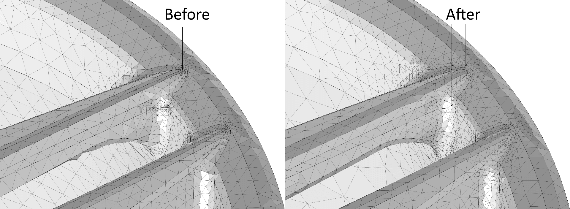
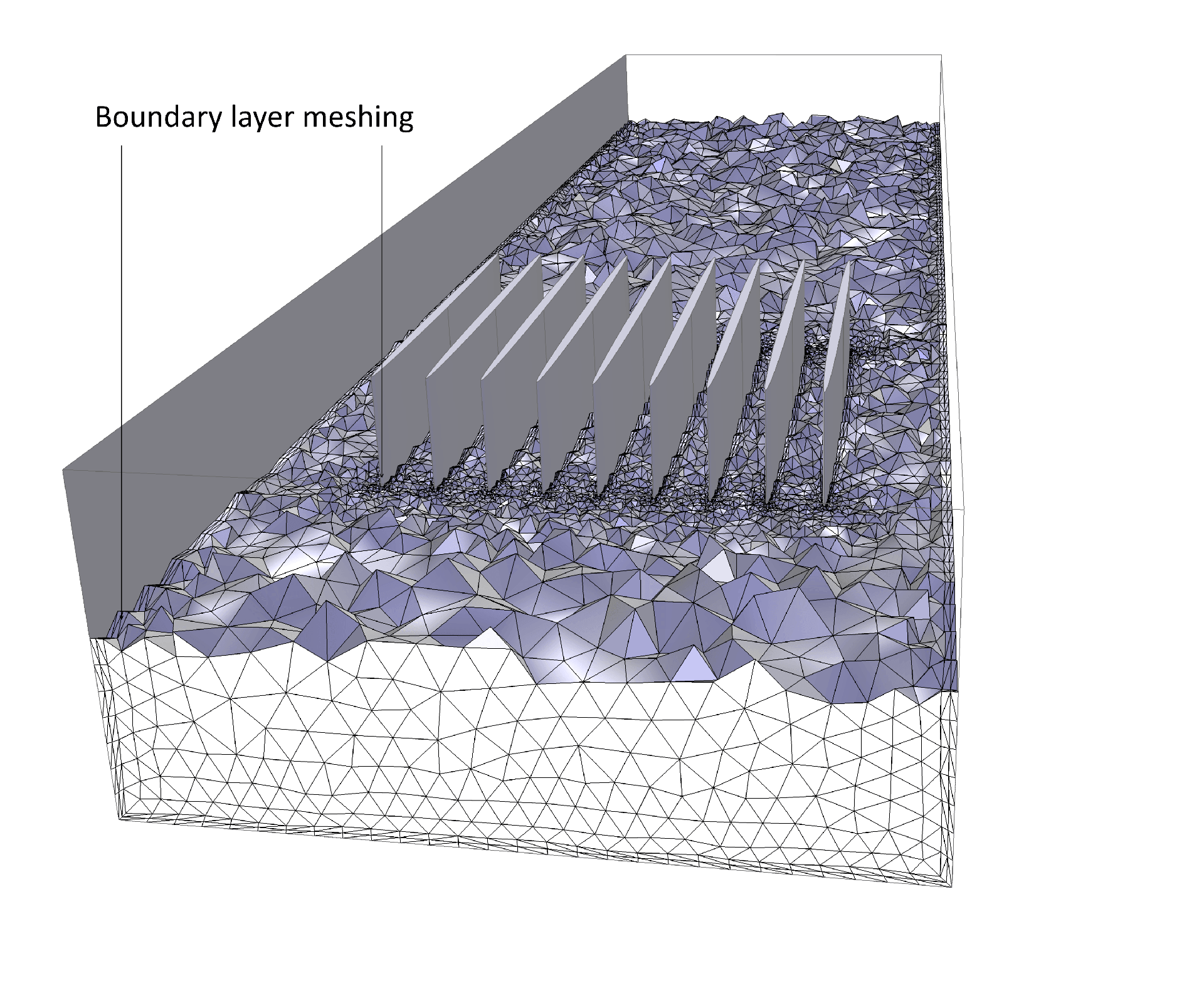 The mesh at the solid surfaces is refined by using boundary layer meshing for fluid flow modeling.
The mesh at the solid surfaces is refined by using boundary layer meshing for fluid flow modeling.
The mesh at the solid surfaces is refined by using boundary layer meshing for fluid flow modeling.
In many cases, different parts of a CAD geometry have to be meshed separately. The model variables have to be matched by the FEA software at the interfaces between the different parts. The matching can be done through continuity constraints (i.e., boundary conditions that relate the finite element discretizations of the different parts to each other). Due to the possible nonlocal character of these conditions, they are often called multipoint constraints.
Meshing is considered to be one of the most difficult tasks of preprocessing in traditional FEA. In modern FEA packages, an initial mesh may be automatically altered during the solution process in order to minimize or reduce the error in the numerical solution. This is referred to as adaptive meshing.
Solution
If creating the mesh is considered a difficult task, then selecting and setting the solvers and obtaining a solution to the equations (which constitute the numerical model) in a reasonable computational time is an even more difficult task. The difficulty is associated with a variety of challenges.
First of all, the discretized model can be very large in terms of algebraic equations. A 3D model can easily have several million degrees of freedom. A central part of the solution process for numerical models originating from the finite element method is to solve a large linear system of algebraic equations. Nonlinear, parametric, eigenvalue, and time-dependent problems are treated with iterative methods, where a sequence of large linear systems are solved.
Large linear systems are, in general, difficult to solve efficiently. Black box methods exist, but they are often too expensive for realistic models. Examples are direct solvers, based on LU factorization methods, or general-purpose iterative methods.
To find a successful and near-optimal alternative, some sort of structure of the underlying system has to be exploited. For multiphysics problems, such a structure might not exist or may be difficult to identify. In such cases, it can be useful to split the problem into its physics constituents for which it is known how to exploit the structure. To accelerate the iterative solution process for linear systems, modern FEA packages use geometric or algebraic multigrid methods.
The nonlinearity of models is another source of problems for FEA solvers. Newton methods use local derivative information to search for better solution candidates, which is only reliable if the current estimate of the solution is close enough to the true numerical solution. In practice, the initial guess for the solution is not always close enough and the Newton method is usually not sufficient to use in such cases. Different simplifications, or relaxations, of the problem may be useful. Instead of the original problem, a simpler nearby problem may be solved to provide a solution candidate. For example, one may neglect certain nonlinearities to obtain a linear problem that can be solved easily. Segregated and continuation solvers are developed for these purposes.
A third class of difficulties encountered by FEA solvers involves the fact that the numerical model might not be stable or, for other reasons, does not give a good approximation to the mathematical model. In these situations, the solution process might be much more difficult than for a more benign and well-behaved numerical model. It may be difficult to detect and understand the reason for this problem. In many cases, the remedy can be to modify the model in some way other than through the solver settings. A better adapted mesh is often an important ingredient in model behavior improvement.
All in all, the options to set up the solvers need to be very flexible and, at the same time, give access to powerful methods. Often, a compromise has to be struck between robustness and performance.
It is always good practice to perturb the numerical model to investigate how sensitive it is. This serves two related purposes: to check if the model is numerically stable and quantify the truncation errors for some significant quantity of interest in the FEA at hand. Usually, but not always, the truncation errors from the finite element discretization dominate the errors in a simulation. For this purpose, a critical derived value in the model can be compared against a typical mesh element size. The computation is then repeated with different meshes (ideally, two other meshes that differ significantly from the current mesh and from each other).
If things are in order with the numerical model, the order of accuracy can be estimated from the comparison. If the order of accuracy is positive, then the difference of the studied quantity between the two finest meshes can serve as an estimate of the truncation error for this quantity. It is not always possible to create several meshes that satisfy all requirements; a comparison between two radically different meshes will then have to serve as a substitute.
A small difference indicates that the numerical model is well-behaved and that the truncation error is small for this quantity. However, if the difference is large, it is more difficult to draw any conclusions. Such differences may be caused by an instability or poor accuracy in both meshes. However, it is possible that the fine mesh solution is accurate, while the coarse mesh solution is poor. Even if the truncation error estimate is uncertain, it can be useful to, at least, rule out the risk that the model is unstable (e.g., by using yet another mesh that is comparable but different to the fine mesh). Other discretization parameters and solver settings, such as tolerances, should also be varied. If the quantity studied changes only to a small extent for all "perturbed" simulations, this is an indication of a stable numerical model.
Results
Analyzing the results from a numerical solver involves investigating 3D plots of the modeled fields, cross-section plots (such as x-y plots), and also evaluating derived values, such as integrals over volumes, surfaces or edges, or values of expressions along edges or in a point.
In older FEA packages, the plots and derived values to be analyzed had to be defined before the solution was ran. Omission of some key definitions means that the solution has to be carried out once again from the beginning. The definition of the expressions and derived values to be analyzed in postprocessing is, therefore, considered a part of preprocessing.
Modern FEA packages allow for the definition of expressions and derived values on the fly, after the solution has been computed. In these packages, the definition of expressions and derived values is part and parcel of postprocessing to drill down on model predictions.
 The generation and analysis of 3D plots, surface plots, x-y plots, and tabulated values from expressions and derived values is proper postprocessing.
The generation and analysis of 3D plots, surface plots, x-y plots, and tabulated values from expressions and derived values is proper postprocessing.
The generation and analysis of 3D plots, surface plots, x-y plots, and tabulated values from expressions and derived values is proper postprocessing.
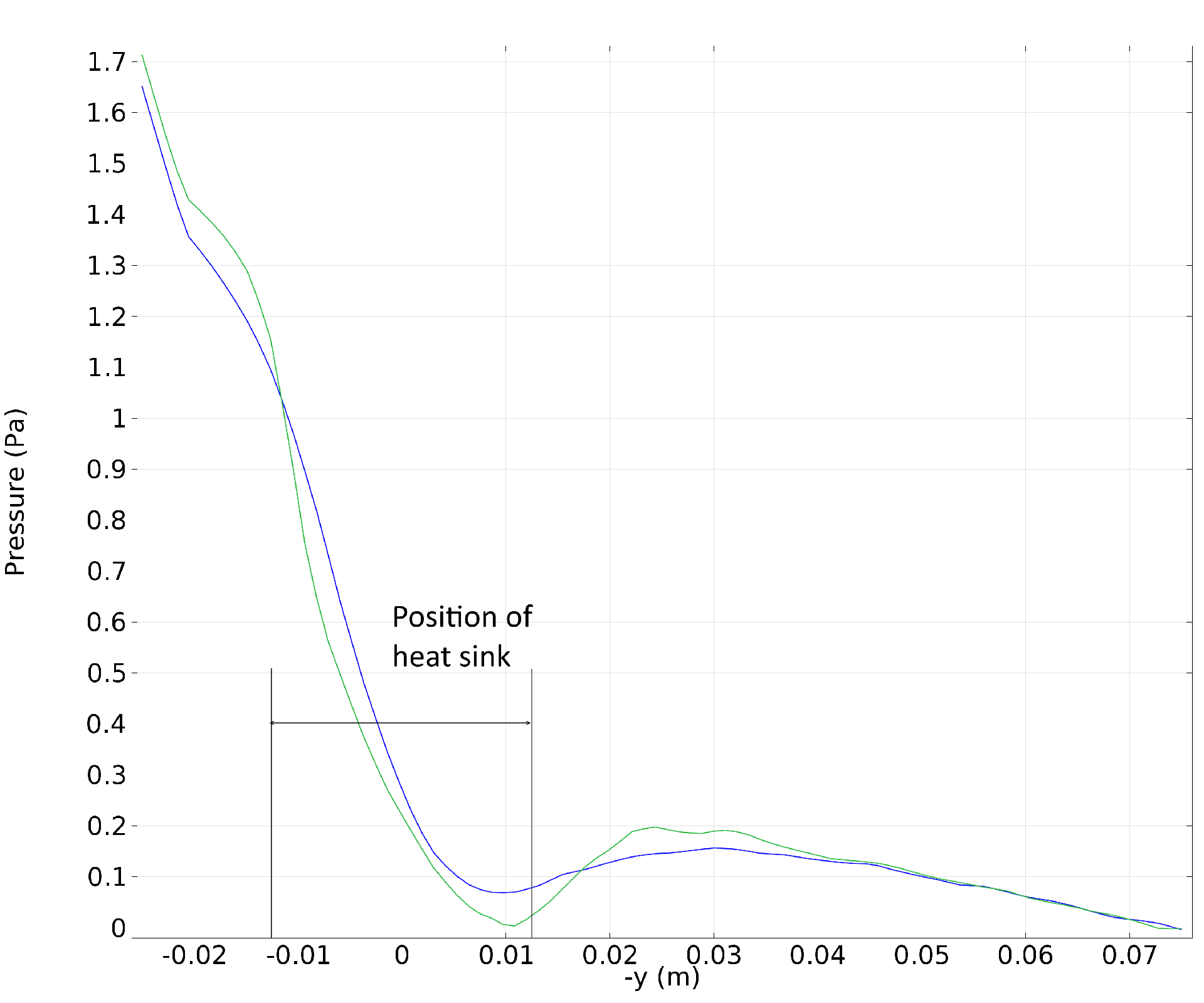 Pressure loss along the direction of the flow at the line at the top of the fin (blue) and at the bottom (green). The pressure loss is slightly larger at the bottom, since the flow has to travel around the relatively large cross section of the heat sink base.
Pressure loss along the direction of the flow at the line at the top of the fin (blue) and at the bottom (green). The pressure loss is slightly larger at the bottom, since the flow has to travel around the relatively large cross section of the heat sink base.
Pressure loss along the direction of the flow at the line at the top of the fin (blue) and at the bottom (green). The pressure loss is slightly larger at the bottom, since the flow has to travel around the relatively large cross section of the heat sink base.
An important task in postprocessing is to estimate the error in the numerical solution. As mentioned above, this can be achieved by solving the numerical model equations for different mesh sizes in order to estimate the convergence of the numerical solution.
Another important part of postprocessing is to estimate the sensitivity of the model to the different data, such as material properties, initial conditions, boundary conditions, loads, constraints, and other input parameters required in the mathematical and numerical models.
Automatic Model Documentation
Once a simulation has been ran, it is important that the input data and the simulation results are summarized in a report that documents the specific session. Modern FEA software can define a report structure, where the user can select which inputs and outputs should be documented. Such reports can then be automatically generated and saved as documentation to be used as a future reference for each simulation.
 First page of a report from a simulation of the heat sink. Once the structure is created, the report is automatically updated for every simulation and can be saved under different names to document simulations. The report contains a problem definition section with domain settings, boundary settings, initial condition, mesh, and number of degrees of freedom. The results contain the derived values and plots that are included in the model file.
First page of a report from a simulation of the heat sink. Once the structure is created, the report is automatically updated for every simulation and can be saved under different names to document simulations. The report contains a problem definition section with domain settings, boundary settings, initial condition, mesh, and number of degrees of freedom. The results contain the derived values and plots that are included in the model file.
First page of a report from a simulation of the heat sink. Once the structure is created, the report is automatically updated for every simulation and can be saved under different names to document simulations. The report contains a problem definition section with domain settings, boundary settings, initial condition, mesh, and number of degrees of freedom. The results contain the derived values and plots that are included in the model file.
FEA Development Trends
The FEA process incorporates many steps, as seen in the overview above. Many details, such as the choice of numerous parameters, which control the solution process, have been successfully automated and do not need much user attention. FEA is much more streamlined today than the software of the last generation and it's available to engineers and smaller enterprises at affordable prices.
However, a lot remains to be done so that FEA potential can provide better engineering designs that can be fully realized. Both algorithms and user interfaces are continuously being improved. An important current trend is to lighten the burden of computational method details on the engineers, designers, and researchers who use FEA for their specific applications. New software interfaces are being developed to help an FEA expert build application-specific tools, together with an application expert, which allows the engineer to concentrate on design tasks, instead of "babysitting" sensitive computations.
The availability of cheap cloud computing resources, when combined with secure means of data transport, will enable intensified computational campaigns in design projects. The past and present of mathematical modeling and FEA software is a success story. The next-generation software will be a significant step. Not only will the numbers be crunched with less engineering effort, the analyses will be more accurate, thus supporting the whole product chain from conception to production. The future for mathematical modeling with FEA software sure does look bright.
 The future looks bright for FEA.
The future looks bright for FEA.
The future looks bright for FEA.
Last modified: February 21, 2017