流体流れ, 熱伝導および質量輸送
An Introduction to Fluid Flow, Heat Transfer, and Mass Transport
The subject of transport phenomena describes the transport of momentum, energy, and mass in the form of mathematical relations[1]. The basis for these descriptions is found in the laws for conservation of momentum, energy, and mass in combination with the constitutive relations that describe the fluxes of the conserved quantities[2]. The most accurate way to express these conservation laws and constitutive relations in continuum mechanics is to use differential equations[3].
Solving the equations that describe transport phenomena and interpreting the results is an efficient way to understand the systems being studied. This methodology is successfully used for studying fluid flow, heat transfer, and chemical species transport in many fields, including:
- Engineering sciences
- Biology
- Chemistry
- Environmental sciences
- Geology
- Material science
- Medicine
- Meteorology
- Physics
Momentum, Energy, and Mass Transport Analogies
The conservation laws for the different transported quantities (momentum, energy, and mass) can be derived from simple principles. Take, for example, a quantity Φ that is conserved in a system where its flux is given by a vector j = (jx, jy, jz). A balance of the quantity Φ may be obtained by looking at each small volume element with dimensions Δx, Δy, and Δz, where the flux, j, is given in quantity per unit area and unit time. The production or consumption term, Rs, is given in quantity per unit volume and unit time.
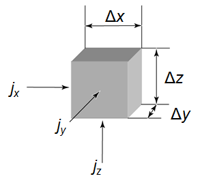
Based on the figure above, the equations for the balance of the quantity are as follows:

Here, jx,x denotes the flux in the x-direction at a position x, and jx,x+Δx is the flux vector in the x-direction at a position x+Δx. The subscripts, t and t+Δt, refer to states at the corresponding times. This equation implies that if there is no production or consumption (Rs = 0), the net flux into or out of the volume element must be balanced by the accumulation or depletion of that quantity over time. Further, if there is no accumulation or depletion over time, then the fluxes into the volume must exactly balance the fluxes out of the volume, so that the total flux into or out of the volume element is zero.
Dividing the above equation by the volume, ΔxΔyΔz, and letting Δx, Δy, and Δz each approach zero, gives the following equation for the quantity Φ:

Letting Δt approach 0 yields:

In order to follow the conservation laws, this balance equation has to be satisfied in every tiny volume element in a continuum (a fluid or solid, for example) in the studied system. This partial differential equation – “partial” since it is expressed as a change along one independent variable at a time (x, y, z, and t are independent variables) – is able to describe the conservation laws of momentum, energy, and mass in modeling and simulations of transport phenomena.
For the conservation of momentum, the conserved quantity is a vector, while the flux term is expressed in a tensor form including the so-called stress tensor. Combining the conservation of momentum, the constitutive equations for the flux of momentum, and the conservation of mass for an incompressible Newtonian fluid yields the Navier-Stokes equations. These equations are the basis for the modeling of fluid flow (CFD) and their solutions describe the velocity and pressure field in a moving fluid. If the conserved quantity is energy, the heat transfer equation in the system can be derived from the conservation equation above.
Finally, let us look at mass transport. Assume that we want to study the composition of a fluid where transport and reactions are present. We can then define and solve the conservation equations for the mass of each species in the fluid. The concentration ci of each species i is the conserved quantity and its flux is denoted by Ni.. Using the conservation equation above gives us the following equation for each species:

If we also assume that the flux is given by diffusion and that Fick’s law defines the constitutive relation for the flux (for a solute in a solvent, for example), we obtain the diffusion-reaction equation often used to model reacting systems with negligible fluid flow:

In this equation, Di denotes the diffusion coefficient of species i in the solution.
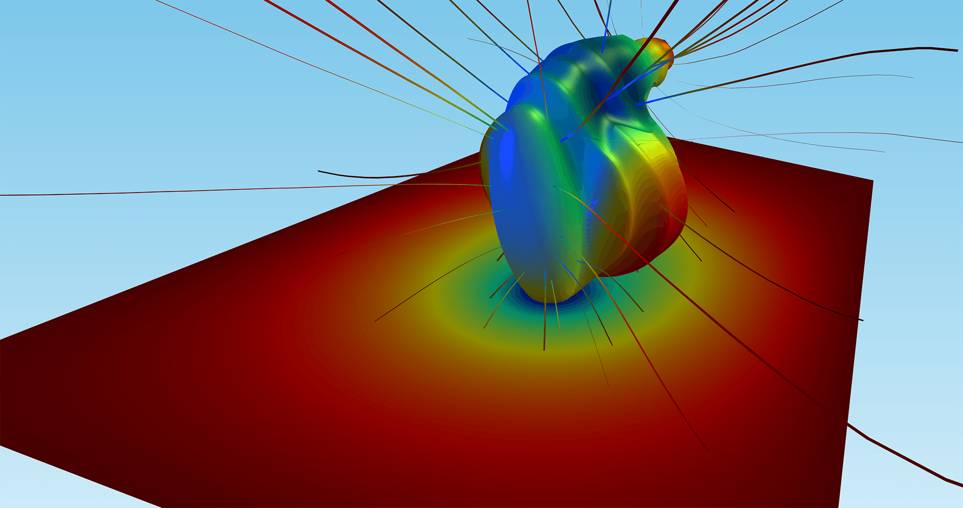
Diffusion in water surrounding a zebra fish embryo and diffusion and reaction of oxygen in the fish embryo's body (reproduced from [4]). Note the high concentration of oxygen in the yolk, where there is hardly any metabolism taking place, only energy storage. Also, insects "breathe" by diffusion. Diffusion-reaction processes are widely used to describe biological systems.
Diffusion in water surrounding a zebra fish embryo and diffusion and reaction of oxygen in the fish embryo's body (reproduced from [4]). Note the high concentration of oxygen in the yolk, where there is hardly any metabolism taking place, only energy storage. Also, insects "breathe" by diffusion. Diffusion-reaction processes are widely used to describe biological systems.
If there is advection, which means that there is a net transport of the whole solution, then we get the transport equation often used in reacting systems where fluid flow is present:

In this equation, u denotes the velocity vector. If there is an electric field E applied on the solution and ions are present, then we obtain the Nernst-Planck equations used in electrochemical systems:

In this equation, zi denotes the valence of species i and ui denotes the mobility of speciesi. The mobility is directly related to diffusivity through the Nernst-Einstein relation. The third term in the flux vector is called the migration term.
The analogy in the conservation of transported quantities is also present in the constitutive relations for the fluxes. For example, transport properties derived from molecular properties yield the viscous term in momentum transport, which is given by Newton's law for fluids; the conduction term in heat transfer, given by Fourier's law for heat transfer; and the diffusion term in mass transport, given by Fick's law for diffusion. The linear relation of the migration term to the electric field parallels Ohm's law, which arises from the transport properties of electrons in metals.
In gases, the transport properties for viscosity, thermal conductivity, and diffusivity are derived from collisions, Brownian motion, and molecular interactions. In liquids, the theory is less general, but still relates molecular momentum, energy, and mass transport properties for a given fluid.
In conclusion, the principle of defining the model equations is straightforward. It is a matter of defining the conservation laws and the relations for how flux can be provoked. It is by solving these equations for a given system over and over again under different conditions, and then studying the results, that we get an understanding of the transport phenomena in the system.
Published: January 14, 2015Last modified: March 22, 2018
References
- R.B. Bird , W.E. Stewart , and E.N. Lightfoot , Transport Phenomena, 2nd edition, John Wiley & Sons, Inc., 2007.
- "Transport Phenomena", Wikipedia.
- R.P. Feynman , R.B. Leighton , and M. Sands , The Feynman Lectures on Physics, Vol II, p. 2-1, The California Institute of Technology, 1989.
- S. Kranenbarg , Oxygen Diffusion in Fish Embryos, Doctoral Thesis, Experimental Zoology, Wageningen University, The Netherlands, 2002.