Modeling Acoustic Ray Tracing: Source with Directivity
In the previous part, we demonstrated the first point ray source method we are using to define loudspeaker reflectivity, Release from Exterior Field Calculation. In this part, we will use the second method, Source with Directivity as an alternative method for defining a point ray source with a speaker's radiation characteristics. This option allows you to use measured data or simulation results from an analysis conducted in a separate model to define the source directivity for ray tracing. Here, we will employ the same model we just created to demonstrate the use of this feature, which enables us to compare the solutions obtained from both methods.
The article "Using Acoustic Ray Tracing to Model Speaker-Room Performance" provides context for this article.
The Source Model
For the Source with Directivity feature, the ray intensity or power is initialized in reference to the actual sound pressure level measured at a reference distance from the source. Therefore, in the source model, we add a second Exterior Field Calculation node and use the Full integral option. This allows us to calculate the actual pressure/sound pressure level at a balloon surface located outside the computational domain at the desired reference distance from the source. Here the exterior field variable is named pext_full to distinguish it from the variable named for the far-field limit case. This is the only change we need to make in the source model.
 A blue plane and a blue hemispherical boundary are shown in the graphics window.
The Full integral option is used in the Exterior Field Calculation 2 node in the source model for calculating the actual pressure/sound pressure level at a finite distance to the source.
A blue plane and a blue hemispherical boundary are shown in the graphics window.
The Full integral option is used in the Exterior Field Calculation 2 node in the source model for calculating the actual pressure/sound pressure level at a finite distance to the source.
The images below display the sound pressure level distribution measured 1 meter from the source, calculated using the full integral exterior field variable. The left image shows the distribution in the xy-plane for the selected frequencies, while the right image presents it in 3D for 2500 Hz.
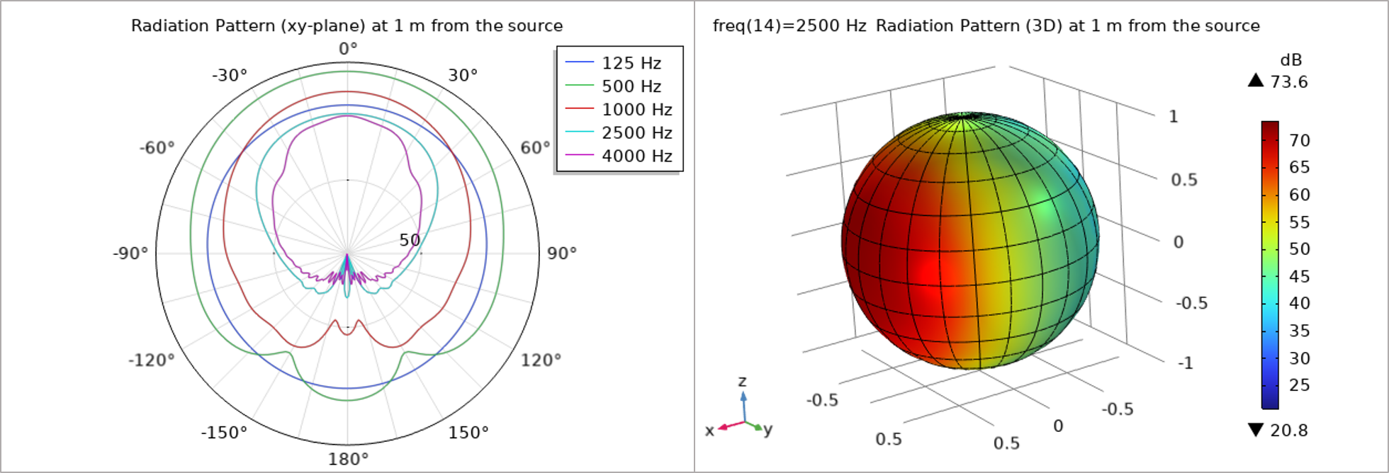 Colored lines for various frequencies are plotted in 2D on the left and a sphere is colored according to the sound pressure level in 3D on the right.
The sound pressure level distribution (1 m from the source) calculated using the full integral exterior field variable.
Colored lines for various frequencies are plotted in 2D on the left and a sphere is colored according to the sound pressure level in 3D on the right.
The sound pressure level distribution (1 m from the source) calculated using the full integral exterior field variable.
The Source with Directivity feature requires balloon interpolation data described in terms of the azimuthal and polar angle defined with respect to the selected coordinate system; therefore, we need to export the data (pressure or sound pressure level) along with the angles describing the location of each evaluation point to a text file in the specified format. In this example, we choose to export pressure (both the real and imaginary parts) at the balloon surface located 1 meter from the source.
In versions 6.3 and later, you can easily add a Radiation Pattern node under Results > Export to export the radiation balloon data, as illustrated in the image below. This helps simplify the process.
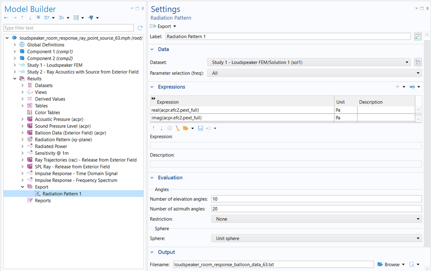 The expressions for the an exported Radiation Pattern are shown.
Version 6.3 introduces a new Radiation Pattern (Export) feature for conveniently exporting radiation balloon data to a text file.
The expressions for the an exported Radiation Pattern are shown.
Version 6.3 introduces a new Radiation Pattern (Export) feature for conveniently exporting radiation balloon data to a text file.
While the process has been simplified in newer versions, older versions can use a Model Method through a Method Call node (see the image below) to facilitate generating and exporting the data for all (or selected) frequencies with desired angle range and resolution. The exported data are saved into one single file including five columns: the first is frequency, which is followed sequentially by the azimuthal angle (phi), the inclination or polar angle (theta), and then the real part and the imaginary part of the exterior field pressure.
 The settings for a Method Call node named RadiationBalloon 1 are shown.
The example in version 6.2 uses a Model Method and Method Call to generate and export the radiation balloon data.
The settings for a Method Call node named RadiationBalloon 1 are shown.
The example in version 6.2 uses a Model Method and Method Call to generate and export the radiation balloon data.
Click here to see the Model Method
int Nf = f.length; //Number of frequencies
int datai = 0; //Row number index in data table
double phi[] = new double[Nphi]; //Azimuth angles vector
double theta[] = new double[Ntheta]; //Incline angles vector
double data[][] = new double[Nf*Nphi*Ntheta][5]; //Data table
String resultTag = "gevbe"; //Results general evaluation tag name
String tableTag = "tblbe"; //Table tag name

//Check if general evaluation node exists
if (model.result().numerical().index(resultTag) >= 0) {
  model.result().numerical().remove(resultTag);
}

//Check if table node exists
if (model.result().table().index(tableTag) >= 0) {
  model.result().table().remove(tableTag);
}

// Iterate i from 0 to Nphi minus 1
for (int i = 0; i < Nphi; ++i) {
  // Repeated N times
  phi[i] = Rphi[0]+i*(Rphi[1]-Rphi[0])/(Nphi-1);
}

// Iterate i from 0 to Ntheta minus 1
for (int i = 0; i < Ntheta; ++i) {
  // Repeated N times
  theta[i] = Rtheta[0]+i*(Rtheta[1]-Rtheta[0])/(Ntheta-1);
}

//Create global evaluation node
model.result().numerical().create(resultTag, "EvalGlobal");
model.result().numerical(resultTag).setIndex("looplevelinput", "first", 0);

//Start timer
long timeStamp = timeStamp();

//Loop over all frequencies and angles to populate data table
for (int i = 0; i < Nf; ++i) {
  for (int ip = 0; ip < Nphi; ++ip) {
    for (int it = 0; it < Ntheta; ++it) {

      double x = x0+r0*Math.cos(phi[ip])*Math.sin(theta[it]);
      double y = y0+r0*Math.sin(phi[ip])*Math.sin(theta[it]);
      double z = z0+r0*Math.cos(theta[it]);

      String x_st = toString(x);
      String y_st = toString(y);
      String z_st = toString(z);
      String f_st = toString(f[i]);
      String phi_st = toString(phi[ip]);
      String theta_st = toString(theta[it]);

      model.result().numerical(resultTag).setIndex("expr", f_st, 0);
      model.result().numerical(resultTag).setIndex("expr", phi_st, 1);
      model.result().numerical(resultTag).setIndex("expr", theta_st, 2);

      //Export real and imaginary part of pressure
      model.result().numerical(resultTag).setIndex("expr", "withsol('sol1',real("+pext_st+"("+x_st+","+y_st+","+z_st+")),setval(freq,"+f_st+"))", 3);
      model.result().numerical(resultTag).setIndex("expr", "withsol('sol1',imag("+pext_st+"("+x_st+","+y_st+","+z_st+")),setval(freq,"+f_st+"))", 4);

      //Export SPL and phase (uncomment if necessary and comment above two lines)
      //model.result().numerical(resultTag).setIndex("expr", "withsol('sol1',20*log10(abs("+pext_st+"("+x_st+","+y_st+","+z_st+"))/sqrt(2)/20e-6[Pa]),setval(freq,"+f_st+"))", 3);
      //model.result().numerical(resultTag).setIndex("expr", "withsol('sol1',arg("+pext_st+"("+x_st+","+y_st+","+z_st+")),setval(freq,"+f_st+"))", 4);

      double dataTemp[][][] = model.result().numerical(resultTag).computeResult();

      for (int ii = 0; ii < 5; ++ii) {
        // Repeated N times
        data[datai][ii] = dataTemp[0][0][ii];
      }
      datai = datai+1;
    }
  }
}

//Stop timer and print compute time to Messages
long compTime = timeStamp()-timeStamp;
String compTime_st = "Export balloon compute time: "+formattedTime(compTime, "h:min:s");
message(compTime_st);

//Export file (default)
if (isFileExport) {
  writeFile("temp:///"+filename, data, false);
  fileSaveAs("temp:///"+filename);
}

//Write to table (optional, not advised for large data sets)
if (isTableExport) {
  model.result().table().create(tableTag, "Table");
  model.result().table(tableTag).label("Table - Radiation Balloon");
  model.result().table(tableTag).comments("Radiation Balloon Data");
  model.result().table(tableTag).setIndex("headers", "freq (Hz)", 0, 1);
  model.result().table(tableTag).setIndex("headers", "phi (rad)", 1, 1);
  model.result().table(tableTag).setIndex("headers", "theta (rad)", 2, 1);
  model.result().table(tableTag).setIndex("headers", "real(p) (Pa)", 3, 1);
  model.result().table(tableTag).setIndex("headers", "imag(p) (Pa)", 4, 1);
  model.result().table(tableTag).addRows(data);

  //Select the table and go back to the method
  ModelEntity origNode = getCurrentNode();
  selectNode(model.result().table(tableTag));
  selectNode(origNode);
}
The Ray Acoustics Model for Using the Source with Directivity Feature
Before setting up the ray acoustics model using the Source with Directivity feature, we need to complete the following two tasks:
1) Import the directivity data using interpolation functions, as seen below. The two functions, named preal and pimag, interpolate the real and imaginary parts of the pressure respectively. You need to enter 3 for Number of arguments since there are three arguments (i.e., frequency and two polar angles) in this case. The Position in file for each function is the position of that function's source data column after the argument columns. Here it should be 1 for preal and 2 for pimag since they are stored at the first and second columns after the three argument columns in the text file.
 The settings for the Interpolation of the balloon pressure are shown.
The interpolation functions defined are based on the exported exterior field pressure.
The settings for the Interpolation of the balloon pressure are shown.
The interpolation functions defined are based on the exported exterior field pressure.
2) Define a coordinate system to reflect the orientation of the speaker. As shown in the image below, a Rotated System feature is used and a value of 180 degrees is given to α to specify the Euler angles because again, the orientation of the speaker is in an opposite direction in the ray tracing model compared to that in the source model.
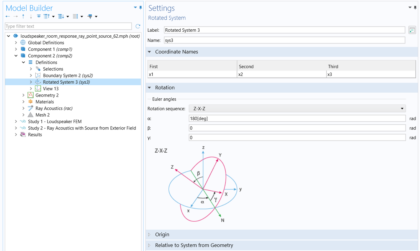 The Rotated System settings window shows how the axis in blue moved to the locations in red.
A Rotated System is defined to reflect the orientation of the speaker in the ray tracing model.
The Rotated System settings window shows how the axis in blue moved to the locations in red.
A Rotated System is defined to reflect the orientation of the speaker in the ray tracing model.
The Point Ray Source Setup
In the same ray acoustics model for demonstrating the Release from Exterior Field Calculation feature, add a Source with Directivity node to the Ray Acoustics physics and use the rotated system and the interpolation functions to specify the directivity of the source in the settings, as shown below. Here we choose the Specify spatial directivity option in the Directivity setting. The 1st argument used for the preal and pimag functions is the study frequency (f0), and the 2nd and 3rd are the built-in variables for the azimuthal (rac.swd1.phi) and polar (rac.swd1.theta) angles. These angles are defined with respect to the selected coordinate system, in this case, the Rotated System 3 (sys3) described above. Here, rac.swd1.theta is the angle between the ray direction vector and the positive z-axis of sys3, while rac.swd1.phi is the angle of the projected ray direction vector in the xy-plane of sys3, measured counterclockwise from the positive x-axis of sys3. The entire expression calculates the sound pressure level in each radiation direction and thus defines the directivity of the ray source.
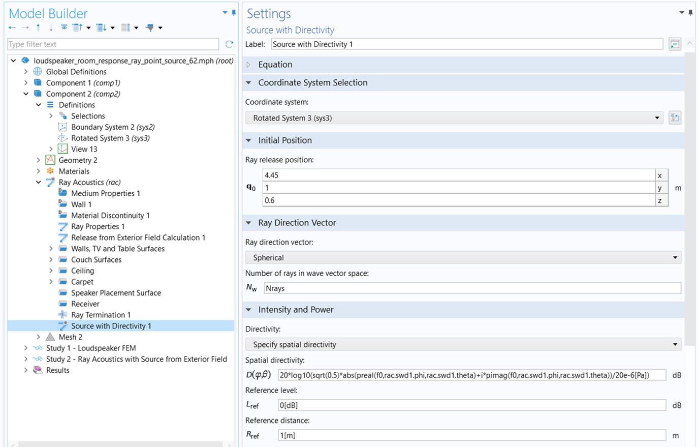 The settings for the Source with Directivity are shown using the rotated system.
The rotated system and the balloon interpolation functions are used to specify the source directivity in the Source with Directivity feature.
The settings for the Source with Directivity are shown using the rotated system.
The rotated system and the balloon interpolation functions are used to specify the source directivity in the Source with Directivity feature.
Note that the Reference distance is specified to be 1[m], which should match the distance of the evaluation surface from the source in the source model. The settings for the ray release position and ray direction vector remain the same, as do the wall conditions and the receiver settings.
Keep in mind that when using a study with the Source with Directivity release feature, the Release from Exterior Field Calculation node is disabled. As a result, the ray frequency specified in the Ray Properties 1 node reverts to the user-defined value f0, which was set earlier.
The Study Setup
Add a new Ray Tracing study and select only the Ray Acoustics physics interface in the Physics and Variables Selection section. In the Output times text field within the Study Settings section, input 0 and 1000 (using the default time unit of millisecond) for the start and final simulation times. Then, enable Modify model configuration for study step (click the check box) and disable the Release from Exterior Field Calculation node (click the node and then the Disable button in the tool bar below), as shown in the top image below. This way, the Release from Exterior Field Calculation node is disabled for the study, and the Source with Directivity node is used for releasing rays. In the Values of Dependent Variables section, simply use the default Physics controlled option for the initial values settings since the directivity data are imported and therefore there is no need to pass solutions from the previous study to the current. Finally, add a Parametric Sweep study node to the current study (Study 3). In the Study Settings, add the parameter f0 and specify its value list to match exactly the 16 frequencies used in Study 1.


The Results
The images below show the ray trajectory at 10 ms (left), and the sound pressure level on the couch surfaces at 1000 ms (right) from the study using Source with Directivity. They are very close to the results obtained from the study using Release from Exterior Field.
 Colored particles are show in a room on the left and the surfaces of the room are colored on the right.
Ray trajectories (left) and SPL plots (right) showing the ray tracing solutions for using the Source with Directivity feature.
Colored particles are show in a room on the left and the surfaces of the room are colored on the right.
Ray trajectories (left) and SPL plots (right) showing the ray tracing solutions for using the Source with Directivity feature.
To conduct impulse response analysis in version up to 6.2, we need to create a Receiver 3D dataset from Study 3 solutions in the same way the Receiver 3D 1 dataset was created from Study 2 solutions. As shown below, the ray dataset automatically generated from Study 3, labeled Ray2 (top), is used to define a receiver dataset named Receiver 3D 2 (bottom). Please note again that in the receiver data settings, you should set Receiver to Receiver(rac/rec1), the receiver defined in the physics, for faster impulse response computation.


We can then conduct impulse response in the same way described earlier. The figure below compares the frequency spectrum of the impulse response at the receiver obtained using the Source with Directivity feature (green curve) to that obtained using the Release from Exterior Field Calculation feature (blue curve). The results are highly consistent, with a maximum deviation of less than 1 dB. Several factors can contribute to the discrepancy observed here, such as the different methods of describing source directivity in the ray acoustics model and the resolution of angles used to export the directivity data for the Source with Directivity feature.
 A 2D plot comparing the Frequency Spectrum of the two point ray source options for different frequencies.
Comparison of the frequency spectrum of the impulse response obtained using the two point ray source options.
A 2D plot comparing the Frequency Spectrum of the two point ray source options for different frequencies.
Comparison of the frequency spectrum of the impulse response obtained using the two point ray source options.
Further Learning
To learn more on how to set up ray acoustics models, download the documentation and MPH-files from the Application Gallery: - Small Concert Hall Acoustics - Chamber Music Hall
このページに関するフィードバックを送信, または サポートに連絡 してください.