私たちがいつも受ける質問は, “特定の電磁気デバイスまたはアプリケーションをモデル化するには, どの COMSOL 製品を使用すればよいですか?”というものです. COMSOL Multiphysics® ソフトウェアのコアパッケージの機能に加えて, 現在, 製品ツリーの電磁気モジュールブランチ内に 6 つのモジュールがあり, その他のフィジックスと結合したさまざまな形式のマックスウェル方程式を扱う残りの製品構造全体に 6 つのモジュールがあります. これらを見て, どのような機能があるかを見てみましょう.
注: このブログは, 2013年9月10日に最初に公開されました. その後, 追加情報と例が追加されて更新されました.
計算電磁気学:マックスウェル方程式
マックスウェル方程式は, 電荷密度 \rho, 電場 \mathbf{E}, 電気変位場 \mathbf{D}, 電流 \mathbf{J}, および磁場強度 \mathbf{H}, 磁束密度 \mathbf{B} を関連付けます:
|
\nabla \cdot \mathbf{D} = \rho
|
\nabla \cdot \mathbf{B} = 0
|
|
\nabla \times \mathbf{E} = -\frac{\partial}{\partial t} \mathbf{B}
|
\nabla \times \mathbf{H} = \mathbf{J} + \frac{\partial}{\partial t} \mathbf{D}
|
これらの方程式を解くには, 境界条件と, \mathbf{E} を \mathbf{D} 場に, \mathbf{J} を \mathbf{E} 場に, \mathbf{B} を \mathbf{H} 場に関連付ける材料構成関係が必要です. さまざまな仮定の下で, これらの方程式は COMSOL 製品内のさまざまなモジュールで解かれ, 他のフィジックスと連成されます.
注: ここで紹介する方程式のほとんどは, 重要な概念を伝えるために省略形で示されています. すべての支配方程式の完全な形式と, 利用可能なさまざまな構成関係をすべて確認するには, 製品説明書を参照してください.
まずはいくつかの概念から始めましょう…
定常状態, 時間領域, 周波数領域?
マックスウェル方程式を解くとき, 計算の負担を軽減するために, 合理的かつ正しい仮定をできるだけ多く行うようにしています. マックスウェル方程式は任意の時間変動入力に対して解くことができますが, 入力と計算された解は定常状態または正弦波的に時間変動すると合理的に仮定できる場合がよくあります. 前者は DC (直流) ケースとも呼ばれ, 後者は AC (交流) または周波数領域ケースとも呼ばれます.
定常状態 (DC) の仮定は, 磁場が時間的にまったく変化しないか, または変化しても重要でないほど無視できるほど小さい場合に成立します. つまり, マックスウェル方程式の時間微分項はゼロであると言えます. たとえば, デバイスが電池に接続されている場合 (電池が著しく消耗するまでに数時間以上かかる場合があります), これは非常に合理的な仮定です. より正式には, 次のように言えます. \frac{\partial \mathbf{B} }{\partial t} = \frac{\partial \mathbf{D} }{\partial t} = 0. これにより, マックスウェル方程式から 2 つの項が直ちに省略されます.
周波数領域仮定は, 系上の励起が正弦波状に変化し, 系の応答も同じ周波数で正弦波状に変化する場合に成立します. 別の言い方をすると, 系の応答は線形であるということです. このような場合, 時間領域で問題を解くのではなく, 次の関係を使用して周波数領域で解くことができます: \mathbf{E}(\mathbf{x},t) = \Re \left( \exp ^{j \omega t }\mathbf{E_c(x)} \right), ここで \mathbf{E}(\mathbf{x},t) は空間および時間で変化する場です. \mathbf{E_c(x)} は空間で変化する複素数値場です. \omega は角周波数です. 離散周波数の集合でマックスウェル方程式を解くことは, 時間領域に比べて計算効率が非常に高くなりますが, 計算要件は, 解く対象となる異なる周波数の数に比例して増加します (ただし, いくつかの注意事項については後で説明します).
時間領域で解く必要があるのは, 解が時間とともに任意に変化するか, 系の応答が非線形である場合です (ただし, これにも例外があり, これについては後で説明します). 時間領域シミュレーションは, 対象の時間範囲の長さと考慮される非線形性に比例して解の計算時間が長くなるため, 定常状態シミュレーションや周波数領域シミュレーションよりも計算が難しくなります. 時間領域で解くときは, 入力信号の周波数成分, 特に存在する重要な最高周波数について考えると役立ちます.
電場, 磁場, またはその両方?
マックスウェル方程式は電場と磁場の両方について解くことができますが, 特に DC の場合はどちらか一方を無視するだけで十分な場合がよくあります. たとえば, 電流の大きさが非常に小さい場合, 磁場も小さくなります. 電流が大きい場合でも, 結果として生じる磁場についてはあまり気にしないかもしれません. 一方, 磁石と磁性材料のみで構成されたデバイスの場合のように, 磁場のみが存在し, 電場が存在しない場合もあります.
ただし, 時間領域と周波数領域では, もう少し注意が必要です. ここで最初に確認したい量は, モデル内の材料の 表皮深さ です. 金属材料の表皮深さは通常, \delta = \sqrt{2/{\omega \mu \sigma} } で近似されます. ここで, \mu は透磁率, \sigma は導電率です. 表皮深さが物体の特性サイズよりもはるかに 大きい 場合, 表皮深さの影響は無視でき, 電場のみを解くことができます. ただし, 表皮深さが物体のサイズと同じかそれより小さい場合, 誘導効果が重要になり, 電場と磁場の両方を考慮する必要があります. モデリングを開始する前に, 表皮深さを簡単に確認することをお勧めします.
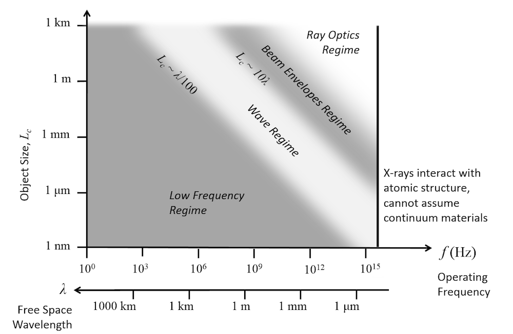
励起周波数を上げると, デバイスの最初の共振を知ることも重要になります. この 基本共振周波数 では, 電場と磁場のエネルギーがちょうどバランスが取れており, 高周波 領域にあると言えます. 共振周波数を推定するのは一般に困難ですが, 経験則として, 特性オブジェクトサイズ L_c と波長 \lambda = c/f を比較します. オブジェクトサイズが波長のかなりの部分 L_c \approx \lambda/100 に近づくと, 高周波領域に近づいています. この領域では, 電力は主に, 導電性材料内の電流ではなく, 誘電体媒体を介した放射によって流れます. これにより, 支配方程式の形が若干異なります. 最初の共振よりも大幅に低い周波数は, 多くの場合, 低周波数領域と呼ばれます.
ここで, これらのさまざまな仮定がマックスウェル方程式にどのように適用されるかを見て, 解くべきさまざまな方程式の集合を示し, それぞれにどのモジュールを使用する必要があるかを確認しましょう.
定常電場モデリング
定常状態を仮定すると, 我々は導電性材料のみ, または完全に絶縁性の材料のみを扱っていると仮定することができます. 前者の場合, 電流はすべての領域に流れると仮定することができ, マックスウェル方程式は次のように書き直すことができます:
この方程式は電位場 V を解き, 電場 \mathbf{E} = -\nabla V と電流 \mathbf{J} = \sigma \mathbf{E} を与えます. この方程式はコアの COMSOL Multiphysics パッケージで解くことができ, ソフトウェアの 入門例 で解かれています. AC/DC モジュール と MEMS モジュール は, コアパッケージの機能を拡張します. たとえば, モデル設定を簡素化する 終端条件 と, 比較的薄い 導電性 領域と 絶縁性 領域のモデル化のための境界条件, および 幾何学的に薄い, 場合によっては多層構造 を通る電流の流れのみをモデル化するための個別のフィジックスインターフェースを提供します.
一方, 物質の誘電率\epsilonを持つ完全に絶縁された媒体内の電場に注目するという仮定の下では, 次の方程式を解くことができます:
これは, 異なる電位にある物体間の誘電体領域の電場強度を計算します. この方程式は, コア COMSOL Multiphysics パッケージでも解くことができます. また, AC/DC モジュールと MEMS モジュールは, たとえば 終端条件, 薄い 誘電体領域 をモデル化するための境界条件, および誘電体材料内の 薄いギャップ などによって機能を拡張します. さらに, これら 2 つの製品は境界要素定式化も提供しており, 同じ支配方程式を解きますが, この 以前のブログで説明されているように, ワイヤーと表面のみで構成されたモデルに対していくつかの利点があります.
時間領域および周波数領域電場モデリング
時間とともに変化する電場をモデル化したい場合, 伝導電流と変位電流の両方が存在するため, AC/DCモジュールまたはMEMSモジュールのいずれかを使用する必要があります. ここでの式は, 上記の最初の式とわずかに異なり, 時間領域の場合は次のように記述されます:
この過渡方程式は, 伝導電流 \mathbf{J}_c = \sigma \mathbf{E} と変位電流 \mathbf{J}_d = \frac{ \partial \mathbf{D} }{\partial t} の両方を解きます. これは, ソース信号が非調和で, 時間の経過に伴うシステム応答を監視する場合に適しています. この例は, 回路内のコンデンサーの過渡モデリング モデルで確認できます.
周波数領域では, 代わりに定常方程式を解くことができます:
この場合の変位電流は \mathbf{J}_d = j \omega \epsilon \mathbf{E} です. この方程式の使用例は, コンデンサーの周波数領域モデリング モデルです.
電場のみをモデル化する場合, 渦電流などの誘導効果は無視されることに注意してください. これらの効果を考慮するには, 時間とともに変化する磁場も解く必要があります.
AC/DC モジュールによる磁場モデリング
定常状態, 時間領域, または低周波領域における磁場のモデリングは, AC/DC モジュール内で処理されます.
磁石や磁性材料のモデルのように, どこにも電流が流れないモデルでは, マックスウェル方程式を簡略化して, 磁気スカラーポテンシャルであるV_mを解くことができます:
この方程式は, 有限要素法または 境界要素法 を使用して解くことができます.
モデルに定常電流が存在する場合, 代わりに磁気ベクトルポテンシャル \mathbf{A} を解く必要があります.
この磁気ベクトルポテンシャルは, \mathbf{B} = \nabla \times \mathbf{A} を計算するために使用され, 電流 \mathbf{J} は, 電気スカラーポテンシャルと電流の前の式を追加することで課すことも, 同時に計算することもできます. このようなケースの典型的な例は, ヘルムホルツコイルの磁場 です.
時間領域に移ると, 次の式を解きます:
ここで \mathbf{E} = -\frac{ \partial \mathbf{A}}{\partial t} .
この方程式は, 伝導電流と誘導電流のみを考慮しており, 変位電流は考慮していません. 電力伝送が主に伝導によって行われ, 放射によって行われない場合は, これは妥当です. この方程式を解くことの大きな動機の 1 つは, 材料の非線形性, たとえば B-H 非線形材料 (この E コアトランスフォーマー の例を参照) がある場合です. ただし, 効果的な H-B 曲線アプローチ を介して B-H 非線形材料を解く別の方法があることに留意してください.
周波数領域に移ると, 支配方程式は次のようになります:
この方程式は伝導電流 \mathbf{J}_c = -j \omega \sigma \mathbf{A} と変位電流 \mathbf{J}_d = \omega^2 \epsilon \mathbf{A} の両方を考慮しており, 波動方程式に非常に似ているように見えます. 実際, この方程式は, 放射が無視できるという仮定の下で, 構造の共振まで, およびその付近を解くことができます. この例が示すとおりです: 3D インダクターのモデリング.
磁場モデリングにおける上記の方程式の使用法のより詳しい紹介については, 電磁コイルモデリングに関する講義シリーズも参照してください.
磁気スカラーポテンシャル方程式とベクトルポテンシャル方程式を混合することも可能で, これは モーターと 発電機のモデリングに応用できます.
磁気ベクトルポテンシャルとスカラーポテンシャルに関する上記の静的, 過渡的, および周波数領域の方程式に加えて, この 超伝導ワイヤー の例のように, 超伝導材料のモデリングに適した磁場に関する別の定式化も存在します.
RF または波動光学モジュールを使用した周波数領域と時間領域での波動方程式モデリング
高周波領域に入ると, 電磁場は波のような性質になります. たとえば, アンテナ, マイクロ波回路, 光導波路, マイクロ波加熱, 自由空間での散乱, および基板上の物体からの散乱のモデリングなどです. 周波数領域におけるマックスウェル方程式のわずかに異なる形式:
この方程式は電界 \mathbf{E} で表され, 磁界は j \omega \mathbf{B} = \nabla \times \mathbf{E} から計算されます. これは, 指定された一連の周波数で解くことも, デバイスの共振周波数を直接解く固有周波数問題として解くこともできます. 固有周波数解析の例には, 密閉空洞, コイル, ファブリ・ペロー共振器のベンチマークがいくつか含まれており, このようなモデルは共振周波数と品質係数の両方を計算します.
指定された周波数の範囲で系の応答を解く場合, 一連の離散周波数で直接解くことができます. この場合, 計算コストは指定された周波数の数に比例して増加します. 代わりに, 単一のコンピューターと クラスターの両方でハードウェア並列処理を利用して, 解を並列化し, 高速化することもできます. また, この ブログで一般的な意味で紹介され, この 導波管アイリスフィルターの例で実証されているように, いくつかの種類の問題の解決を加速する周波数領域モーダルソルバーと適応周波数スイープ (漸近波形評価とも呼ばれる) ソルバーもあります.
RFまたは波動光学モジュールを使用して時間領域で解く場合は, AC/DCモジュールの以前の方程式と非常によく似た方程式を解きます:
この方程式は, 磁気ベクトルポテンシャルを解きますが, 時間における 1 次導関数と 2 次導関数の両方を含むため, 伝導電流と変位電流の両方を考慮します. これは, 光学非線形性, 分散性材料, および 信号伝播のモデリングに適用できます. 時間領域の結果は, この例に示されているように, 高速フーリエ変換ソルバーを使用して周波数領域に変換することもできます.
これらの方程式の計算要件は, メモリに関しても懸念事項です. 対象のデバイスとその周囲の空間は有限要素メッシュによって離散化され, このメッシュは波を解像できるほど細かくなければなりません. つまり, 少なくともナイキスト基準を満たす必要があります. 実際には, これは, 動作周波数に関係なく, 約 10 x 10 x 10 波長のドメインサイズが, 64 GB の RAM を搭載したデスクトップコンピューターでアドレス指定可能な上限を表すことを意味します. ドメインサイズが大きくなると (または周波数が大きくなると), メモリ要件は, 解く対象となる 3 次波長の数に比例して大きくなります. つまり, 上記の方程式は, 特性サイズが対象の最高動作周波数での波長の 10 倍以下である構造に適しています. ただし, この制限を回避する方法が 2 つあります.
波長よりもはるかに小さい物体の周囲の波のような場を解く方法の 1 つに, 陽的時間発展 定式化があります. これは, はるかに少ないメモリを使用して解くことができる, 時間依存のマックスウェル方程式の異なる形式を解きます. これは主に線形材料モデリングを目的としており, 背景場における物体からの広帯域散乱を計算する場合など, いくつかのケースでは魅力的です.
周波数領域で解かれる特定の種類の光導波構造には別の選択肢があり, 電場が伝播方向に非常にゆっくりと変化することが知られています. このような場合, 波動光学モジュールのビームエンベロープ法が非常に魅力的になります. このインターフェースは, 次の方程式を解きます:
ここで, 電場は \mathbf{E} = \mathbf{E_e} \exp \left (-i \phi \right) であり, \mathbf{E_e} は電場の包絡線です.
追加の場 \phi は, いわゆる位相関数であり, 少なくとも近似値で既知でなければならず, 入力として指定する必要があります. 幸いなことに, 多くの光導波の問題では, これはまさに当てはまります. 1 つだけ, または 2 つのビームエンベロープ場を同時に解くことができます. このアプローチの利点は, 使用できる場合, このセクションの冒頭で示した全波方程式よりもメモリ要件がはるかに低いことです. このアプローチの他の使用例としては, 方向性結合器 のモデルや, 光学ガラスの自己集束 のモデリングなどがあります.
AC/DC モジュール, RF モジュール, 波動光学モジュールの選択
AC/DCモジュールとRFモジュールの境界線は少し曖昧です. 自分自身にいくつかの質問をしてみると役に立ちます:
- 私が作業しているデバイスは大量のエネルギーを放射していますか? 共鳴を計算することに興味がありますか? そうであれば, RF モジュールの方が適しています.
- デバイスは, 最高動作波長での波長よりもはるかに小さいですか? 主に磁場に興味がありますか? そうであれば, AC/DC モジュールの方が適しています.
これらの境界線上にいる場合は, 両方の製品を含めることも合理的です.
RF モジュールと波動光学モジュールのどちらにするか決めるには, アプリケーションについて考える必要があります. 時間領域と周波数領域におけるマックスウェル方程式の完全波形に関しては, 機能面で多くの重複がありますが, 境界条件には若干の違いがあります. マイクロ波デバイスのモデリングに適用可能な, いわゆる 集中ポート および 集中要素境界条件があり, これらは RF モジュールのみに含まれています. また, ビームエンベロープの定式化は波動光学モジュールのみに含まれていることにも留意してください.
材料特性に関しては, 2 つの製品には異なる材料ライブラリが付属しています. RF モジュールは一般的な誘電体基板データを提供し, 波動光学モジュールには光学および IR バンドの 1,000 を超えるさまざまな材料の屈折率が含まれています. これとその他の利用可能な材料ライブラリの詳細については, こちらのブログをご覧ください. もちろん, デバイスモデリングのニーズについて具体的な質問がある場合は, お問い合わせください.
これらのモジュール間のおおよその境界線の概要を以下の図に示します.
光線光学モジュールによる光線追跡
波長の何千倍もの大きさのデバイスをモデル化する場合, 有限要素メッシュで波長を分解することはできなくなります. このような場合, 光線光学モジュールで幾何光学アプローチも提供しています. このアプローチは, マックスウェル方程式を直接解くのではなく, モデリング空間を通る光線を追跡します. このアプローチでは, 均一な自由空間ではなく, 反射面と誘電体ドメインのみをメッシュ化する必要があります. これは, レンズ, 望遠鏡, 大型レーザーキャビティ, および 構造熱光学性能 (STOP) 解析 のモデリングに適用できます. この チュートリアルモデル に示されているように, 完全波動解析の出力と組み合わせることもできます.
マルチフィジックスモデリング
COMSOL Multiphysics の強みの 1 つは, マックスウェル方程式を単独で解くことに加え, 複数の物理現象が結合している問題を解くことです. 最も一般的なものの 1 つは, マックスウェル方程式と温度の結合で, 温度上昇が電気的 (および熱的) 特性に影響します. このような種類の電熱問題に対処する方法の概要については, この ブログ を参照してください.
構造変形を電場と磁場に結び付けることもよくあります. これは単に 変形を伴う場合もありますが, 圧電, 圧電抵抗, または 磁歪 材料応答, または 応力光学 応答を伴う場合もあります. MEMS モジュールには, 印加電場によってデバイスにバイアスをかける 静電駆動共振器 専用のユーザーインターフェースがあります. 電流モデリングのコンテキストでは, 構造接触と 接触部品間の電流 の流れも考慮できます.
ただし, 温度と変形だけでなく, 電流のマックスウェル方程式を化学プロセスと組み合わせることもできます. これは, 電気化学, バッテリデザイン, 電気めっき, 腐食解析 の各モジュールで扱われます. プラズマモジュール では, プラズマ化学と組み合わせることもできます. また, 粒子追跡モジュール を使用すると, 電場と磁場を通じて荷電粒子を追跡できます. 最後に (今のところは!), 半導体モジュール では, ドリフト拡散方程式を使用して電荷輸送を解きます. これらの各モジュールは, それ自体がトピックであるため, ここですべてについて説明するつもりはありません.
もちろん, これらのモジュールについてさらに詳しく話し合いたい場合や, 関心のあるデバイスにどのように適用できるかを知りたい場合は, 下のボタンからお気軽にお問い合わせください.
コメント (0)