

In many engineering situations, we can assume that excitations on the system of interest and the responses are sinusoidal over time. When this assumption holds, we can use a so-called frequency-domain analysis, which leads to some very efficient solution techniques. Let’s go over a few basic concepts and the conditions under which we can make this assumption, while exploring various solution approaches to take.
Time-Harmonic Loads in Engineering and Science
Solid mechanics, acoustics, electromagnetics… These are just some of the engineering disciplines where we can often assume that there are sinusoidal excitations. An imbalanced wheel on a car, for example, leads to sinusoidally time-varying forces that cause the vehicle’s structure to vibrate at the same frequency as the rotation of the wheel. In acoustics, a loudspeaker membrane is driven at one or several frequencies, causing sound waves of the same frequencies to radiate. Similarly, in electromagnetics, power transmission lines operate at a constant frequency; cellphone antennas broadcast electromagnetic waves over a discrete range of frequencies; and lasers output nearly monochromatic, single-frequency light. Despite relating to completely different disciplines, the modeling approaches that you need to know about for each of these cases are surprisingly similar.
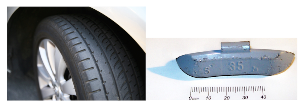
Left: An unbalanced tire is just one example where time-harmonic loads can occur. Image licensed by CC BY 2.0, via Flickr Creative Commons. Right: A trim weight from a car rim.
The partial differential equations that govern these various cases all have the same general form:
(1)
M u_{tt} + C u_t + \nabla \cdot (-K \nabla u) = F &\text { on } \Omega \\
\mathbf{n} \cdot (K \nabla u) + Au = f &\text{ on } \Gamma_1 \\
u = g &\text{ on } \Gamma_2
\end{align}
where u=u(\mathbf{x},t) is the space- and time-varying field of interest (i.e., displacement for a structural problem or pressure for an acoustic problem). The terms M, K, and C represent different material properties, and are usually termed the mass, stiffness, and damping terms, respectively. The term F=F(\mathbf{x},t) denotes the distributed loads on the domain. There are also always a set of boundary conditions that represent the loads, f=f(\mathbf{x},t), and constraints, g=g(\mathbf{x},t), on the system. Boundary loads are specified via the Robin boundary condition, which contains the term A that denotes a boundary absorption or boundary impedance that can be zero. These loads, f, and constraints, g, can either be zero (homogeneous) or nonzero (nonhomogeneous) boundary conditions.
Let’s take a look at the simplest case of the above equation, a simple harmonic oscillator, which is shown in the diagram below.
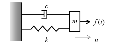
A simple harmonic oscillator where a spring and damper connect a mass to a rigid wall. A time-varying applied force causes the mass to oscillate back and forth.
Now if we also have a set of initial conditions u(\mathbf{x},t=0)=u_0, then we can compute the displacement response of this system over time. The plot below shows the displacement of the mass with the applied load, f(t)=\sin(\omega t), and initial condition, u_0=0. Under these conditions, the mass begins to oscillate back and forth starting from zero. After some initial start-up time, the displacement becomes periodic; it repeats sinusoidally with constant angular frequency, \omega, and will be independent of the initial conditions.
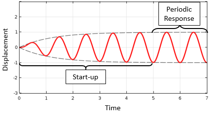
The response of a simple harmonic oscillator to a sinusoidal excitation. Starting from initial conditions of zero, the displacement eventually becomes periodic in time.
There may be much more data here than we really need. For example, we might only be interested in the total start-up time rather than the time evolution during the start-up period. Further, after the start-up period, we might only care about the displacement magnitude. Solving such a problem in the time domain is therefore not truly necessary; we can instead turn this into a so-called frequency-domain problem.
Frequency-domain analysis, however, relies on two important assumptions. First, all time-varying loads and constraints on the system must vary sinusoidally at the same fixed frequency. Second, all loads, constraints, and material properties must be independent of the solution. Under these two assumptions, we can infer that the solution takes the form:
which can be differentiated with respect to time and put into our original governing partial differential equation, giving us:
(2)
-\omega^2 M \tilde u + j \omega C \tilde u+ \nabla \cdot (-K \nabla \tilde u) = \tilde F & \text { on } \Omega \\
\mathbf{n} \cdot (K \nabla \tilde u) + A \tilde u = \tilde f &\text{ on } \Gamma_1 \\
\tilde u = \tilde g &\text{ on } \Gamma_2
\end{align}
which provides the frequency-domain form of our governing equation. Note that the field will be complex valued, and thus contains information about the solution magnitude and phase. This partial differential equation and the boundary conditions are linear, making it very straightforward to solve, as described in our earlier blog post on solving linear static finite element models. Let’s now delve more deeply into the various solution techniques for these types of problems.
Analyzing Problems in the Frequency Domain
The COMSOL Multiphysics® software includes a suite of different algorithms that are appropriate for solving the above equation (Eq. (2)). The most straightforward approach is the frequency-domain solver. This solver takes, as inputs, a single frequency or discrete range of frequencies to simulate.
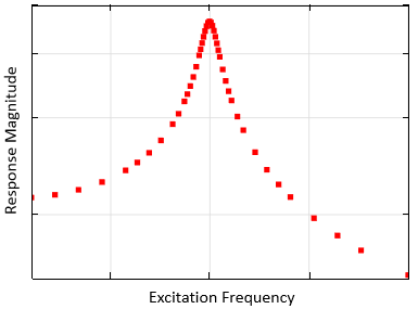
We can, for example, solve our simple harmonic oscillator problem from earlier at a range of excitation frequencies and get a plot similar to the one shown below, which illustrates the displacement magnitude for different excitation frequencies. Regardless of the physics involved, the frequency response will always look similar to the curve below. There will be a maximum in the response vs. frequency curve that corresponds to a resonant frequency of the system. The response on either side of this maximum falls off, and the bandwidth for full width at half maximum can be used to compute Q, the quality factor. The quality factor is particularly useful as it can be related to the start-up time of the system described earlier.
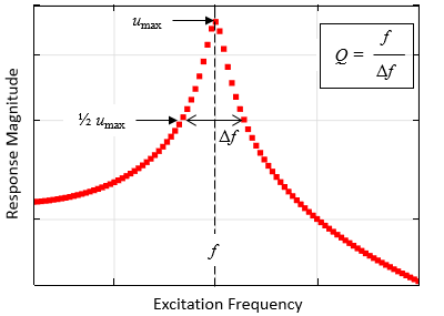
Plot representing the response of a harmonic oscillator to a sinusoidal load in the frequency domain, solved at a set of discrete frequencies. Resonant frequencies and quality factors can be estimated from such a plot.
When solving such problems using the frequency-domain solver, the COMSOL Multiphysics software sequentially solves for each specified excitation frequency. The solution time will therefore increase in proportion to the number of frequencies that are being solved. There are two approaches that you can use to improve solution time: the Cluster Sweep option available with the Floating Network License or the asymptotic waveform evaluation (AWE) solver.
When using the Cluster Sweep option, the software will automatically subdivide the list of frequencies into separate ranges. Each one of these ranges is then solved on a different computational node on a cluster. The advantage here is that you can greatly parallelize the calculation, using as many cluster nodes as you want. You can even set up your model to use a different mesh for each frequency range — an advantageous element if you have very wide band excitation. The software will automatically reassemble the solutions computed on the various nodes of the cluster within a single model. The plot below shows how a frequency sweep is broken into intervals and solved on different nodes of a cluster. You can learn more about cluster computing here on the COMSOL Blog.
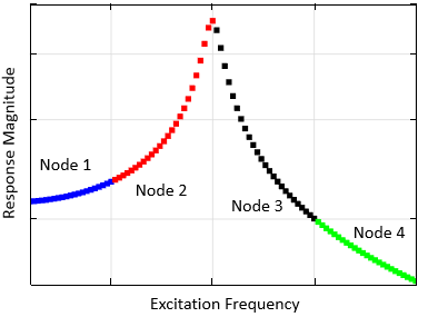
The same frequency sweep as earlier, but with different frequency ranges solved on different nodes of a cluster.
When using the AWE solver, the software will search through the frequency range of interest and successively add calculation points at discrete frequencies within the interval to get a good resolution of the response versus frequency curve. This approach is shown in the plot below. Note how the AWE solver solves for more points around resonance and less points where the response varies gradually with frequency. Such an approach can be combined with the Cluster Sweep option.
The AWE solver introduces additional calculation points in the range where the response changes significantly with frequency.
All of the solution approaches discussed so far give us similar response curves, albeit with different solution time requirements. These solutions are useful for understanding how a system will respond under different excitation frequencies. As shown earlier, we can also use such curves to estimate the resonant frequencies and quality factors of the system. In fact, sometimes these are the only two quantities of interest. This brings us to yet another solution approach known as an eigenfrequency solver.
When solving an eigenfrequency problem, the software is actually solving a slightly different model than the one described by the governing partial differential equation shown earlier. Since we are interested in the natural frequencies of resonance, all nonhomogeneous loads and constraints are changed to their homogeneous (zero magnitude) form:
(3)
-\omega^2 M \tilde u + j \omega C \tilde u+ \nabla \cdot (-K \nabla \tilde u) = 0 & \text { on } \Omega \\
\mathbf{n} \cdot (K \nabla \tilde u) + A \tilde u = 0 &\text{ on } \Gamma_1 \\
\tilde u = 0 &\text{ on } \Gamma_2
\end{align}
When this form of the governing equation is solved, the so-called eigenvalues, \lambda = -j \omega + \delta, of the system are computed. These complex-valued eigenvalues give us the resonant frequencies, f=\omega/2\pi, and the quality factors, Q=f/2\delta. Complex-valued eigenvalues arise due to loss in the system, meaning a nonzero damping term, C, or a complex-valued mass, M, stiffness, K, or absorption, A, term. If there is no loss, then the quality factor is infinite and the software only returns the resonant frequencies. Also returned is the field solution, \tilde u, which can be used to visualize the behavior of the system at resonance. This solution is often referred to as the mode shape or eigenmode.
Let’s look at some sample results from an eigenfrequency analysis of a very simple structural problem: a slender beam pinned at either end. The resonant frequencies and mode shapes of the in-plane bending modes of the beam are plotted below.
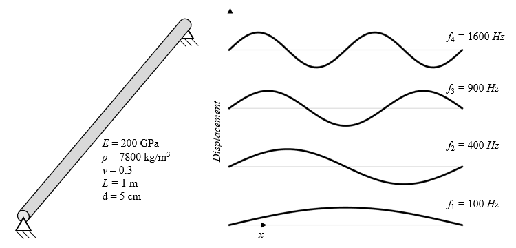
The first four resonant frequencies and mode shapes of a pinned circular beam.
These eigenvalue results can actually be used in yet another study type known as a frequency-domain modal study — a so-called two-step study. In the first study step, a user-specified number of eigenfrequencies and mode shapes are computed. In the second step, a linear combination of these eigenvalue solutions are used to reconstruct the frequency-response behavior. This approach becomes more accurate as more eigenvalues are used. You can see this in the plot below, which compares a sweep using the frequency-domain solver to the results of the frequency-domain modal solver with different numbers of participating eigenvalues.
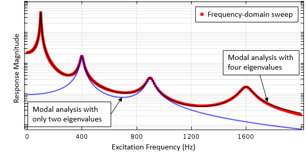
Comparison of a frequency-domain sweep and frequency-domain modal study using a different number of eigenvalues.
Closing Remarks on Modeling the Harmonic Excitations of Linear Systems
Modeling the harmonic excitations of linear systems is an important step in many analysis problems. Today, we have introduced the various solution algorithms that COMSOL Multiphysics offers for solving such models. You will want to keep all of these techniques in mind, as different models will benefit from different algorithms.
But what about nonlinear systems? These systems respond very differently to harmonic excitations, including the creation of lower or higher harmonics. As we will highlight in an upcoming blog post, there are a number of powerful tools available at your fingertips that can be used to address these complex cases. Stay tuned!
Explore Various Applications of Modeling the Harmonic Excitations of Linear Systems
- Want to try out modeling the harmonic excitations of linear systems in COMSOL Multiphysics on your own? Browse this list of tutorials to find the one that best suits your engineering focus:
- Various Analyses of an Elbow Bracket, a structural mechanics tutorial that features frequency-domain, eigenfrequency, and frequency-domain modal analyses
- Helmholtz Resonator Analyzed with Different Frequency Domain Solvers, an acoustics tutorial that includes frequency-domain, eigenfrequency, and frequency-domain modal analyses
- RF Coil, a wave electromagnetics tutorial that features frequency-domain and eigenfrequency analyses
- Evanescent Mode Cylindrical Cavity Filter, a wave electromagnetics example that includes frequency-domain and AWE analyses
- Cascaded Rectangular Cavity Filter, a wave electromagnetics tutorial that features frequency-domain and frequency-domain modal AWE analyses
- Read a related blog post: Methods that Accelerate the Modeling of Bandpass-Filter Type Devices
- Have additional questions in regards to this topic? Feel free to reach out and contact us today

Comments (4)
praveen kumar
October 3, 2017How am I get this model description pdf file?
Walter Frei
October 3, 2017Hello Praveen,
The images here are for illustrative purposes, there are no specifically documented models that go along with these images. Should you have any difficulties using any of the solvers described in this article, please of course reach out to your COMSOL Support Team.
Enver Salkim
April 10, 2019Thank you for the post.
I would like to apply my continuous biphasic current to the terminal of each electrode:
To generate biphasic waveform based on a function by defining upper and lower levels.
My question is how can I apply this function to the ”terminal boundary ” of the electrode in Electric Settings and how to generate a continuous function based on specific frequency?
Thank you for your valuable help in advance.
Kind regards,
Enver
Daniel Giraldo
April 13, 2020Hello, I need to apply a harmonic force at the bottom of a cylinder, but the force has to be rotational. How to define that?
I tried the “Rotational frame” Domain force, but it doesn’t seem to be working. Under the boundary loads, there is nothing like a rotational load.