Modeling with PDEs: Global ODEs and DAEs Interface
Here in Part 6 of this course on modeling with partial differential equations (PDEs) in COMSOL Multiphysics®, you will learn how to solve time-dependent ordinary differential equations (ODEs) and differential-algebraic equations (DAEs) that have no space dependency and hence no association with a mesh or geometry. For this purpose, you can use the Global ODEs and DAEs interface. Such equations are also known as initial value problems. We will also cover linear and nonlinear equations, including systems of equations.
Table of Contents
- Global ODEs and DAEs
- Solving an ODE for a Forced Mass-Spring-Damper System
- Solving a System of ODEs
- Solving a System of Nonlinear ODEs
- Plotting Phase Portraits
- Differential-Algebraic Systems
- Coupling PDE Models with ODEs
- The Lorenz Equation System
- Further Learning
Global ODEs and DAEs
Just as in the case of PDEs, if you have a common application that requires modeling an ODE as an initial value problem, you might find a user-friendly, built-in interface in one of the add-on products. To discover which built-in interfaces are available, start a new model and, in the Select Space Dimension window, select the 0D option. The term 0D is used for initial value problems that do not have any spatial dependency.
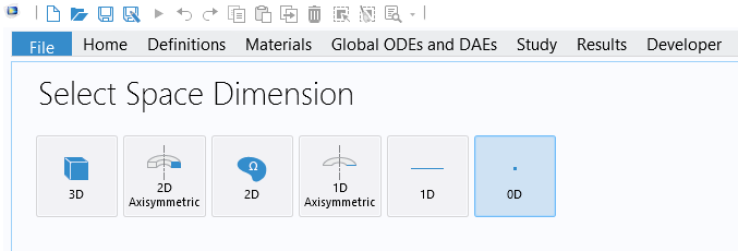
The 0D option.
On the following Select Physics page, you will find a list of available 0D interfaces, as shown in the figure below. To see a complete list of these interfaces, you will need access to various add-on products.
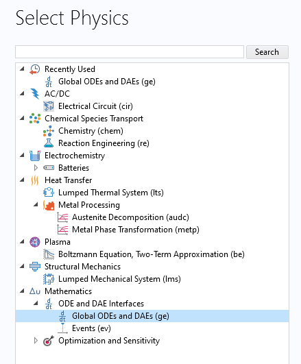
The built-in 0D physics interfaces for modeling ODEs that are initial value problems.
In the figure above, the general-purpose Global ODEs and DAEs interface is highlighted. This is the interface you should select if you want to solve your own ODE or system of ODEs. This interface can also be used if you have a differential-algebraic system of equations, which is a mix of differential and algebraic equations.
Solving an ODE for a Forced Mass-Spring-Damper System
As an easy example to start with, we will look at how we can solve the following second-order initial value problem for a classical forced mass-spring-damper system:

This way of writing a differential equation uses Leibniz's notation.
We can more compactly write this as:

This is known as Lagrange's notation.
Yet another option is Newton's notation:

Here, we will use Lagrange's notation.
The forced mass-spring-damper system is an equation in a time-dependent variable,  , representing the displacement from an equilibrium position of a point with mass,
  . The coefficient
  represents damping, and
  is a spring constant. The right-hand-side function
  represents an external forcing function. Associated with a second-order ODE are two initial conditions:


For more information on the mass-spring-damper model, see https://en.wikipedia.org/wiki/Mass-spring-damper_model.
As a concrete example, we will simulate a mass-spring-damper system with the following parameters:


Assuming you have selected the Global ODEs and DAEs interface, as a final step in the Model Wizard, select a Time Dependent study, as shown below.
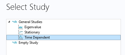
A Time Dependent study is needed for solving an initial value problem.
This will make the Global Equations interface available, as shown in the figure below.
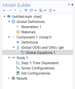
The mathematics interface for ODEs is called Global Equations.
Before defining the equation, create the following global parameters:
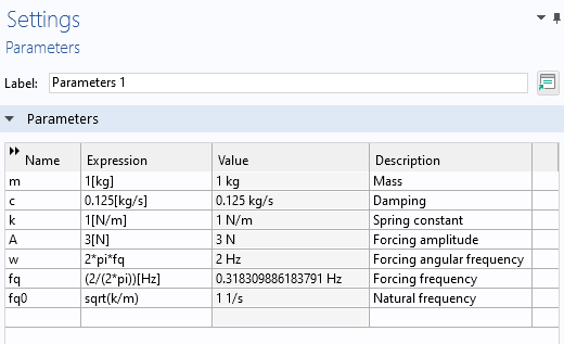
The parameters used for the mass-spring-damper system.
In the user interface, you can use the syntax ut and utt for the first and second derivatives, respectively.
The Global Equations interface requires that we enter the equation on the form:

To adapt the equation to the format required by the user interface, we rewrite the equation slightly as:

so that in all we have:

where the choice of sign here is a convention used in COMSOL®. The convention is that an external (generalized) force acting on a system should enter the equations with a positive sign.
Note that the interface will also accept nonlinear ODEs on implicit form. As the form of the function  implies, an ODE can be defined using a mathematical expression that involves the solution variable, its first- and second-order time derivatives, and an explicit dependency on the time variable t.
In the Global Equations interface, you can now enter the following:
- Name:
u - Equation f(u,ut,utt,t):
A*cos(w*t)-m*utt-c*ut-k*u - Initial value:
u(0)=2 - Initial value:
u'(0)=0 - Dependent variable quantity, Displacement:
m - Source term quantity, Force:
N
In the figure below, these settings have been entered in the user interface:
The Global Equations settings for the mass-spring-damper ODE.
The next step is to define the time interval that we would like to solve for.
In the Model Builder, select the Study>Step 1: Time Dependent node. Change the last time in the expression for Output times to 50. The range(0,0.1,50) syntax means that the solver will output results in intervals of 0.1 s from 0 s to 50 s. These are not the times that the solver is using in its time-stepping algorithm. The algorithm is adaptive and will take more, or sometimes less, time steps than what is specified as Output times depending on the behavior of the equation and the set tolerance.
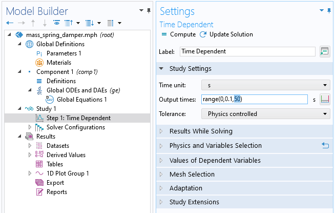
The Output times settings for solving between 0 and 50 seconds.
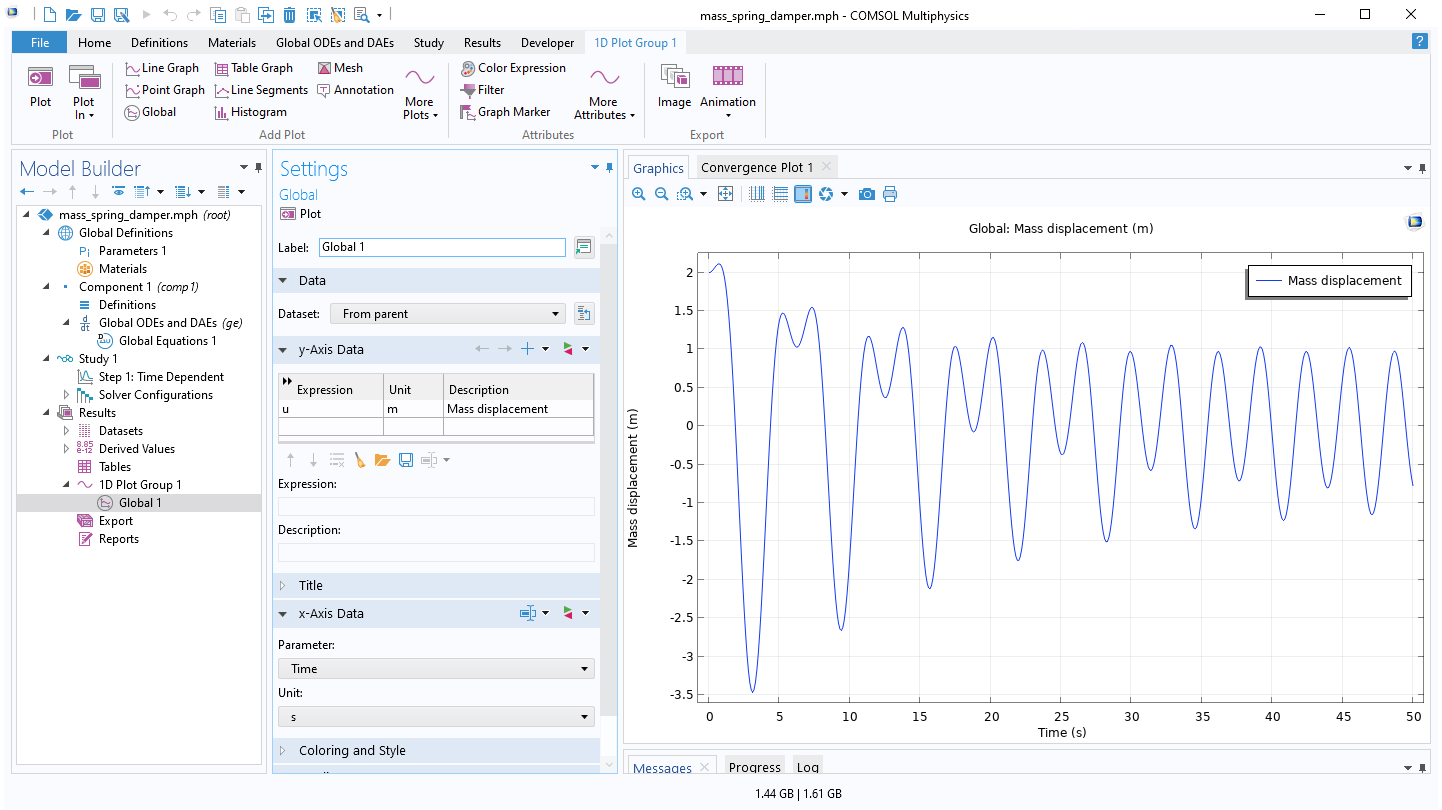
Click Compute to solve. The default plot shows the solution versus time.
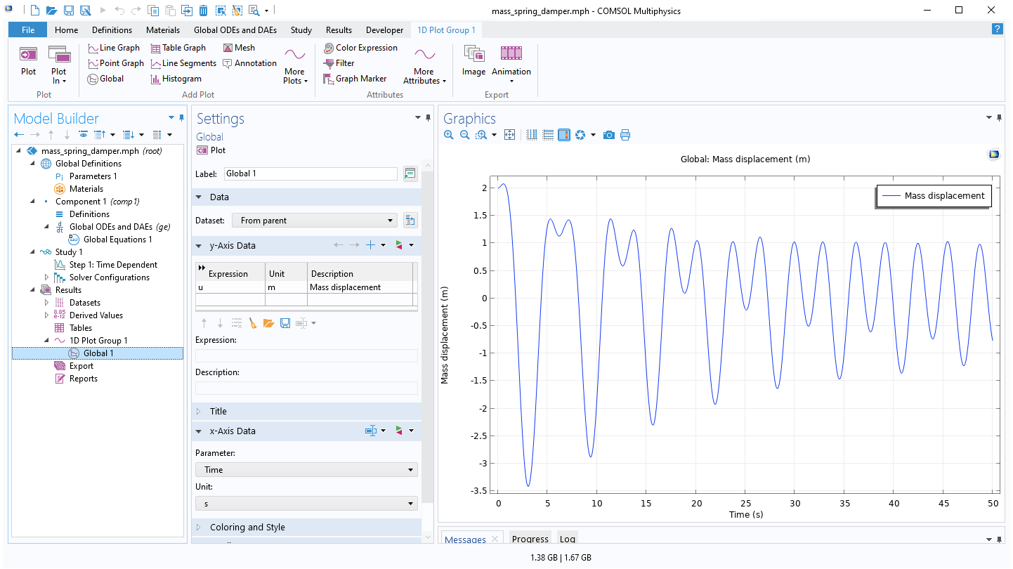 The Model Builder with a Global plot selected, the corresponding settings, and the Graphics window showing the mass displacement.
The solution to the mass-spring-damper ODE between 0 and 50 seconds.
The Model Builder with a Global plot selected, the corresponding settings, and the Graphics window showing the mass displacement.
The solution to the mass-spring-damper ODE between 0 and 50 seconds.
To get a sense of the level of accuracy of the solution, you can lower the tolerance. In the Time Dependent Settings window, change the Tolerance option from Physics controlled to User controlled, and set the Relative tolerance value to 0.0001 (or 1e-4), as shown in the figure below.

The Relative tolerance settings for the Time Dependent study.
The solution changes slightly, as shown in the figure below.
 The Model Builder with a Global plot selected, the corresponding Settings window, and the Graphics window showing the updated mass displacement.
The solution to the mass-spring-damper ODE with a lower solver tolerance.
The Model Builder with a Global plot selected, the corresponding Settings window, and the Graphics window showing the updated mass displacement.
The solution to the mass-spring-damper ODE with a lower solver tolerance.
You can even create a parametric sweep over varying tolerance values, as shown in the figure below.
 The Model Builder with a Global plot selected, the corresponding settings, and the Graphics window showing different mass displacement results.
The solution to the mass-spring-damper ODE with a sweep over successively lower solver tolerances.
The Model Builder with a Global plot selected, the corresponding settings, and the Graphics window showing different mass displacement results.
The solution to the mass-spring-damper ODE with a sweep over successively lower solver tolerances.
Note that the corresponding files are available for download.
We may also be interested in the frequency content of the solution. To display the frequency spectrum in the original mass-spring-damper model (without the tolerance sweep), in the Global plot Settings window, change the Parameter option in the x-Axis Data section to Discrete Fourier transform. Then change the Show option to Frequency spectrum. This plot is shown in the figure below:
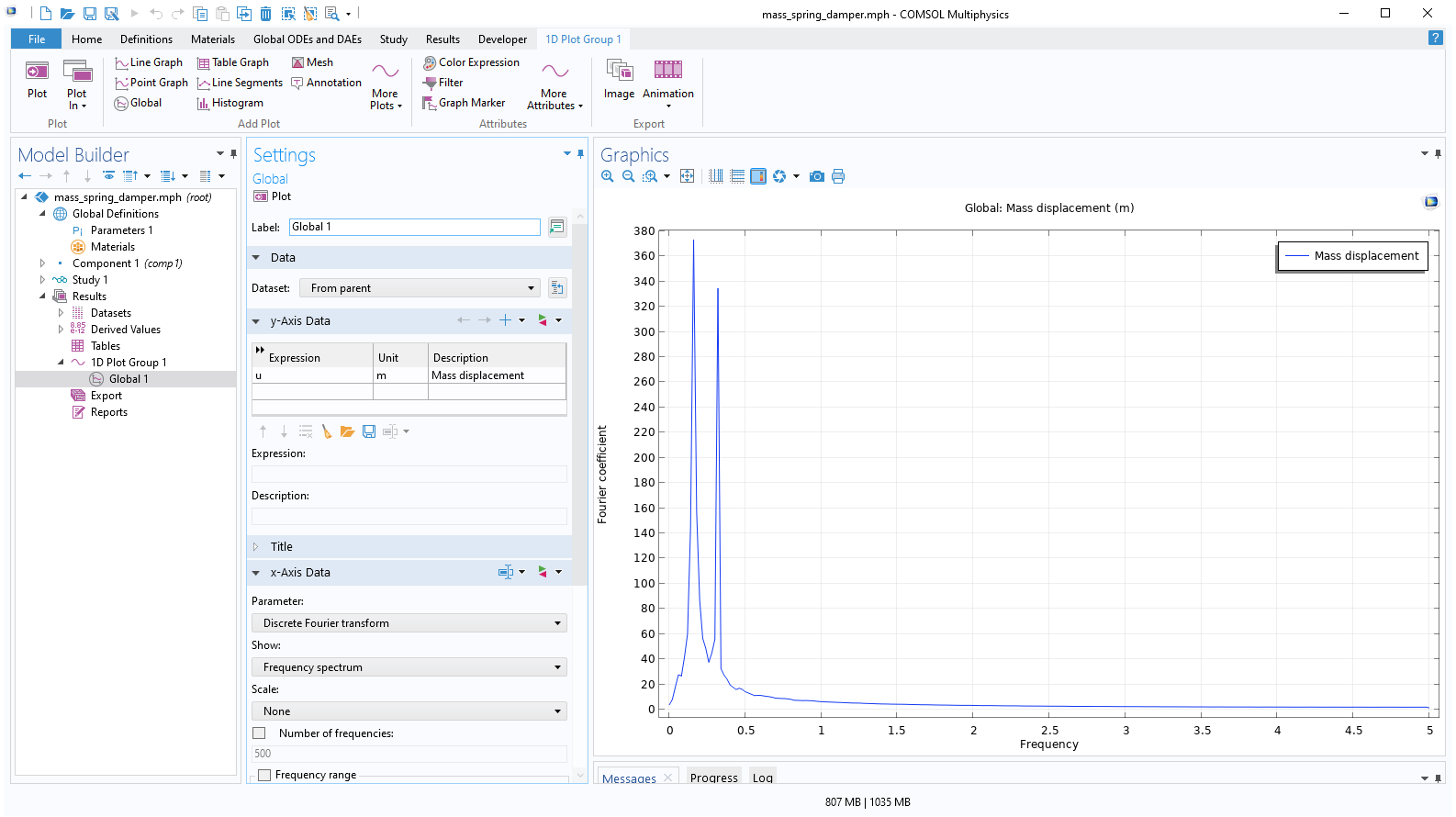 The Model Builder with a Global plot selected, the corresponding Settings window, and the Graphics window showing frequency versus Fourier coefficient.
The frequency spectrum of the mass-spring-damper model.
The Model Builder with a Global plot selected, the corresponding Settings window, and the Graphics window showing frequency versus Fourier coefficient.
The frequency spectrum of the mass-spring-damper model.
You can plot the axes on a logarithmic (log) scale by clicking the x-Axis Log Scale and y-Axis Log Scale buttons in the Graphics toolbar. This gives the following plot:
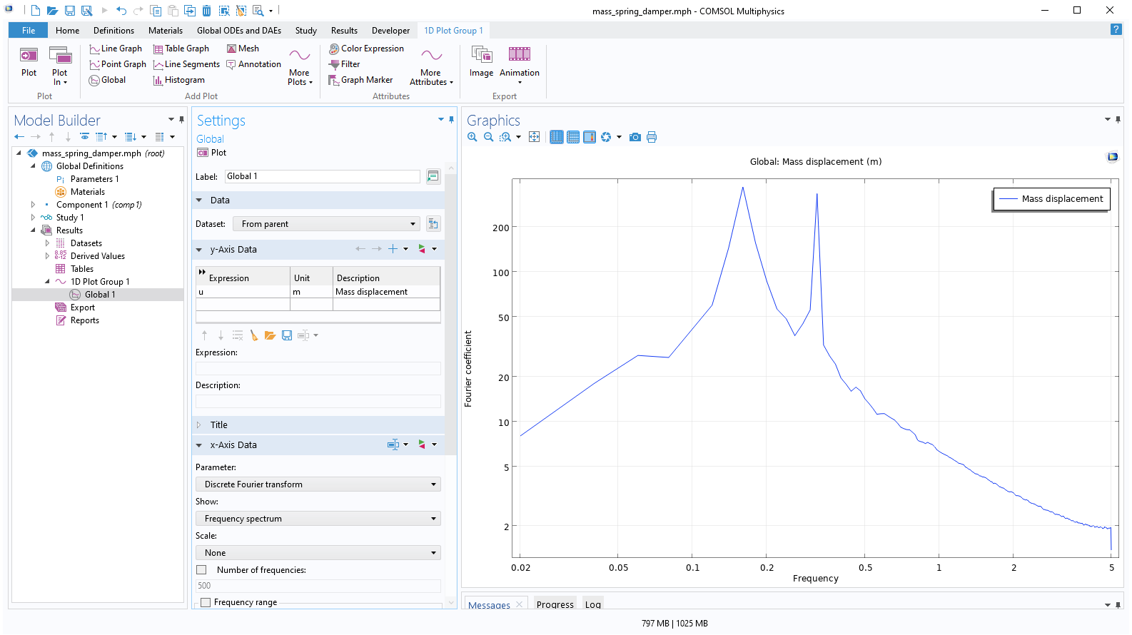 The Model Builder with a Global plot selected, the corresponding settings, and the Graphics window, with the graph plotted with a log scale.
The frequency spectrum of the mass-spring-damper model, plotted using log scale.
The Model Builder with a Global plot selected, the corresponding settings, and the Graphics window, with the graph plotted with a log scale.
The frequency spectrum of the mass-spring-damper model, plotted using log scale.
We see that there are two frequency peaks at 0.16 Hz and 0.32 Hz. Note that if you solve for a longer time period, there will be a sharp spike corresponding to the forcing frequency since it determines the steady-state periodic solution.
Solving a System of ODEs
The Global ODEs and DAEs interface can also be used to solve systems of ODEs. Within chemical engineering it is common to solve systems of ODEs with hundreds, sometimes thousands, of equations. The Chemical Reaction Engineering Module has specialized modeling features for entering such systems. Within electrical engineering you might likewise have large ODE systems when modeling electrical circuits. This is applicable to the Electrical Circuits interface, which is available in several of the add-on products, including the AC/DC Module.
Here, we will look at a simple two-variable system — a system-version of the mass-spring-damper equation. You can rewrite the second-order mass-spring-damper equation as two first-order equations by introducing the velocity,  , of the point mass as a new degree of freedom:

The resulting system can be written as two first-order equations:


There are several different ways that we can enter this system in the user interface. We can simply add the equation for the velocity in the second row of the Global Equations interface, as shown in the figure below.
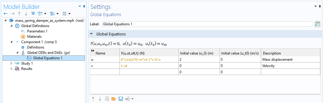 The Model Builder with the Global Equations interface selected and the corresponding Settings window.
The system of differential equations that is equivalent to the scalar mass-spring-damper differential equation.
The Model Builder with the Global Equations interface selected and the corresponding Settings window.
The system of differential equations that is equivalent to the scalar mass-spring-damper differential equation.
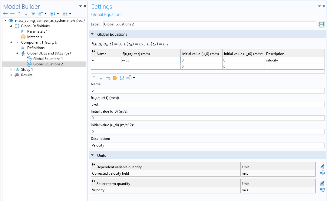
This system will solve correctly; however, if we do it this way, we run into a problem with handling the units. The fact that we now have inconsistent units is indicated by the yellow-orange coloring of the equations. If we want consistent unit handling we instead need to add a second Global Equations interface and change the Dependent variable quantity and Source term quantity units to m/s. This is shown in the figure below.
The second differential equation in the velocity variable used for rewriting the second-order mass-spring-damper differential equation as a system of first-order differential equations.
Solving this system of first-order equations will give us the same solution as when we solved it as a scalar second-order equation.
We can also plot the solution in the phase plane where we plot the displacement, u, on one axis and the velocity, v, on the other axis. This is a 2D plot, and to accomplish this we need to first create a 2D dataset. Right-click the Results > Datasets node and, under More 2D Datasets, select Grid 2D, as shown in the figure below.
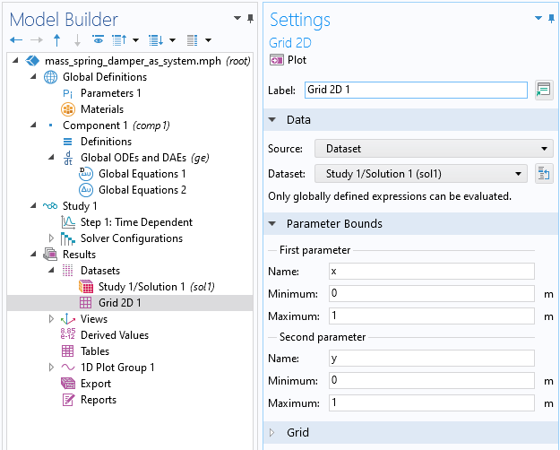
The Grid 2D dataset used to create a phase plane plot.
We do not need to change the settings for the Grid 2D dataset since we will plot quantities that have a global variable scope.
Next, right-click the Results node and select a 2D Plot Group. Right-click this 2D Plot Group and select Point Trajectories, which is available under More Plots. In the Point Trajectories Settings window, enter u and v for the x-expression and y-expression, respectively, as shown in the figure below.
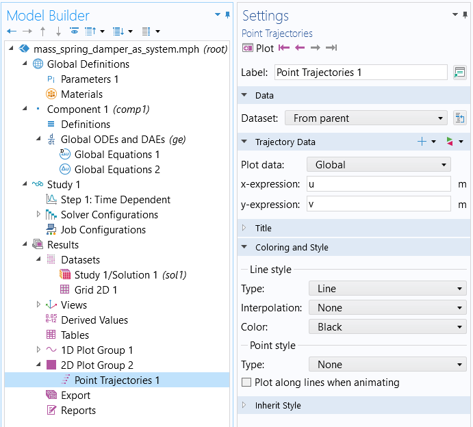
The Point Trajectories settings used for the phase plane plot.
Next, clear the Plot dataset edges check box in the 2D Plot Group settings, as shown below.

The Plot dataset edges are cleared for the Point Trajectories plot.
We now get the following phase-plane plot of the solution:
 The Model Builder with the Point Trajectories plot selected, the corresponding settings showing the plot data, and the Graphics window showing the plot.
The phase-plane plot for the mass-spring-damper differential equation.
The Model Builder with the Point Trajectories plot selected, the corresponding settings showing the plot data, and the Graphics window showing the plot.
The phase-plane plot for the mass-spring-damper differential equation.
We can get a better feeling for the behavior of the solution if we solve the ODE up to 200 s, instead of the current 50 s.
Change the Output times setting to range(0,0.01,200) and compute. This result in the following solution:
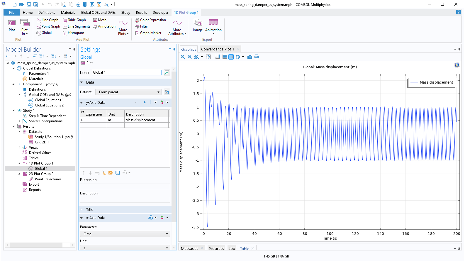 The Model Builder with the Global plot selected, the Settings window with the y-Axis Data section expanded, and the Graphics window showing the mass displacement.
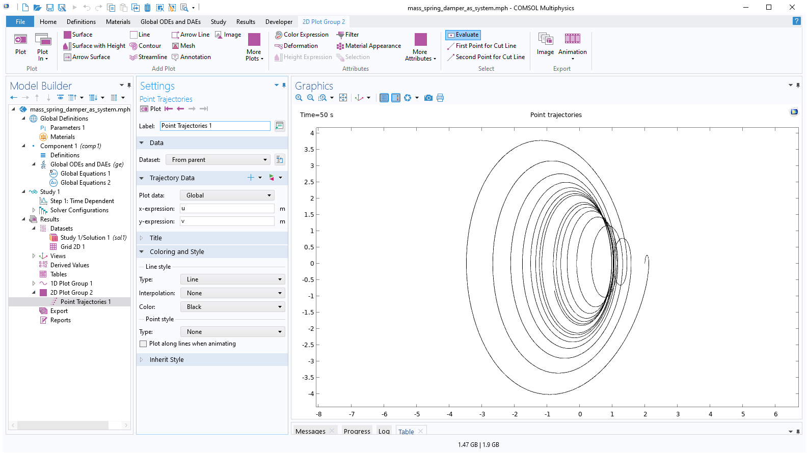
The solution stabilizes to a sinusoidal form determined by the frequency of the forcing function. For c=0.125[kg/s], the corresponding phase-plane plot looks like this:
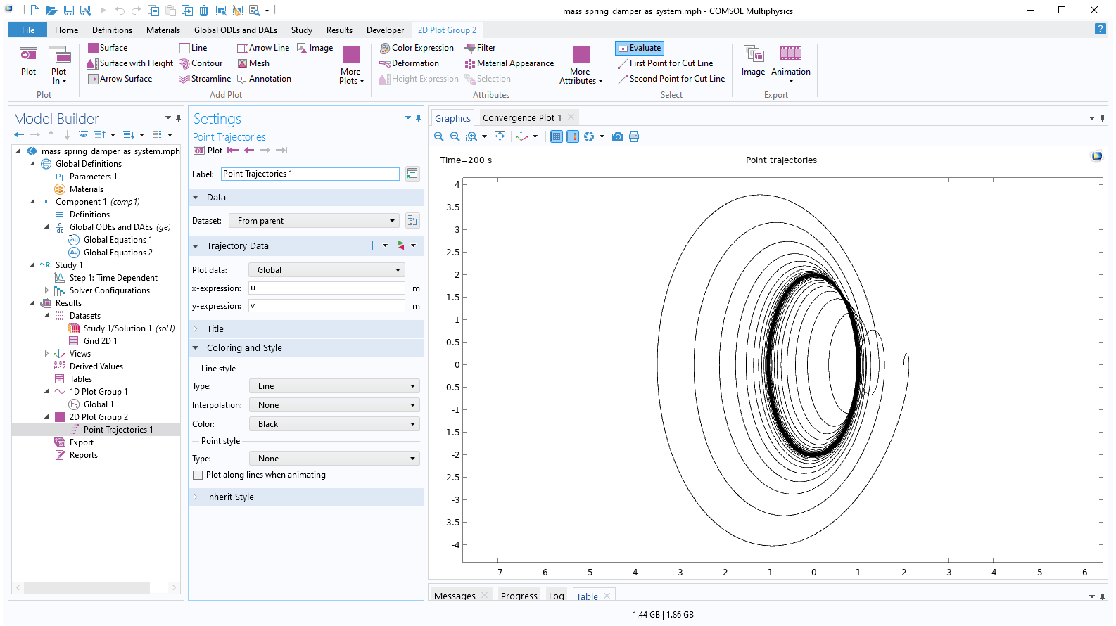 The Model Builder with Point Trajectories selected, the corresponding settings, and the Graphics window with the phase-plane plot.
The stable solution orbit is reflected by the darker region in the phase-plane plot.
Note that you can also generate a phase-plane plot for the previous scalar mass-spring-damper equation by entering ut instead of v in the Point Trajectories plot. However, the variable ut will then be represented by a lower-order approximation than u, so the phase-plane plot will look smoother if we instead use the system where the dependent variables u and v will have the same discretization order.
Solving a System of Nonlinear ODEs
The Global ODEs and DAEs interface is not limited to solving linear equations, such as the mass-spring-damper system. We can enter virtually any type of nonlinearity in the equations. A classical nonlinear extension of the mass-spring-damper system type of equation is to add a nonlinear gain or damping term, as follows:

Here, we change the sign of the damping coefficient and multiply it by a factor,  . This coefficient causes gain if
  is small and causes damping if is large. In this way, the equation has an interesting interplay between damping and gain. This equation has been extensively studied and is called the van der Pol oscillator. It has commonly been used to model oscillations in vacuum tubes. However, in our example we will model the van der Pol equation as a continuation of the mass-spring-damper system, even though the physical interpretation is not straightforward in this case.
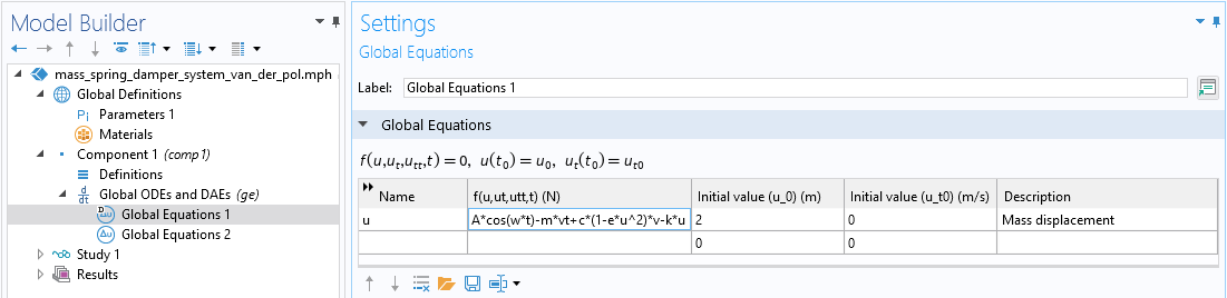
To enter this equation, we can either modify the second-order mass-spring-damper equation or the first-order system of equations. Here, we will modify the first-order system, as follows:

The first of these equations is shown in the figure below, using the same sign convention as in the earlier example.
 A close-up of the Model Builder with the Global Equations interface selected and a close-up of the Global Equations table in the Settings window.
The differential equation for the van der Pol oscillator, entered in the Global Equations interface.
The coefficient e is used to generate a consistent unit and is defined as shown below:
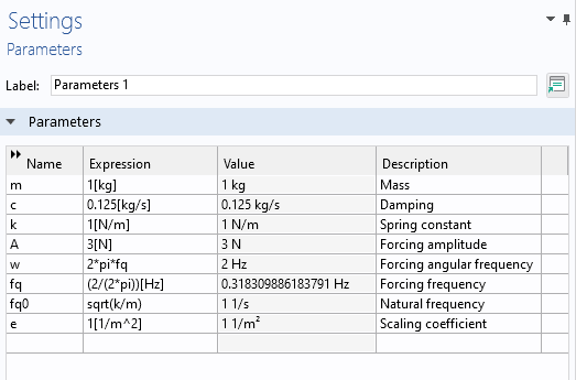
The parameters for the van der Pol oscillator differential equation.
Solving this, using Output times set to range(0,0.01,200), gives the following solution:
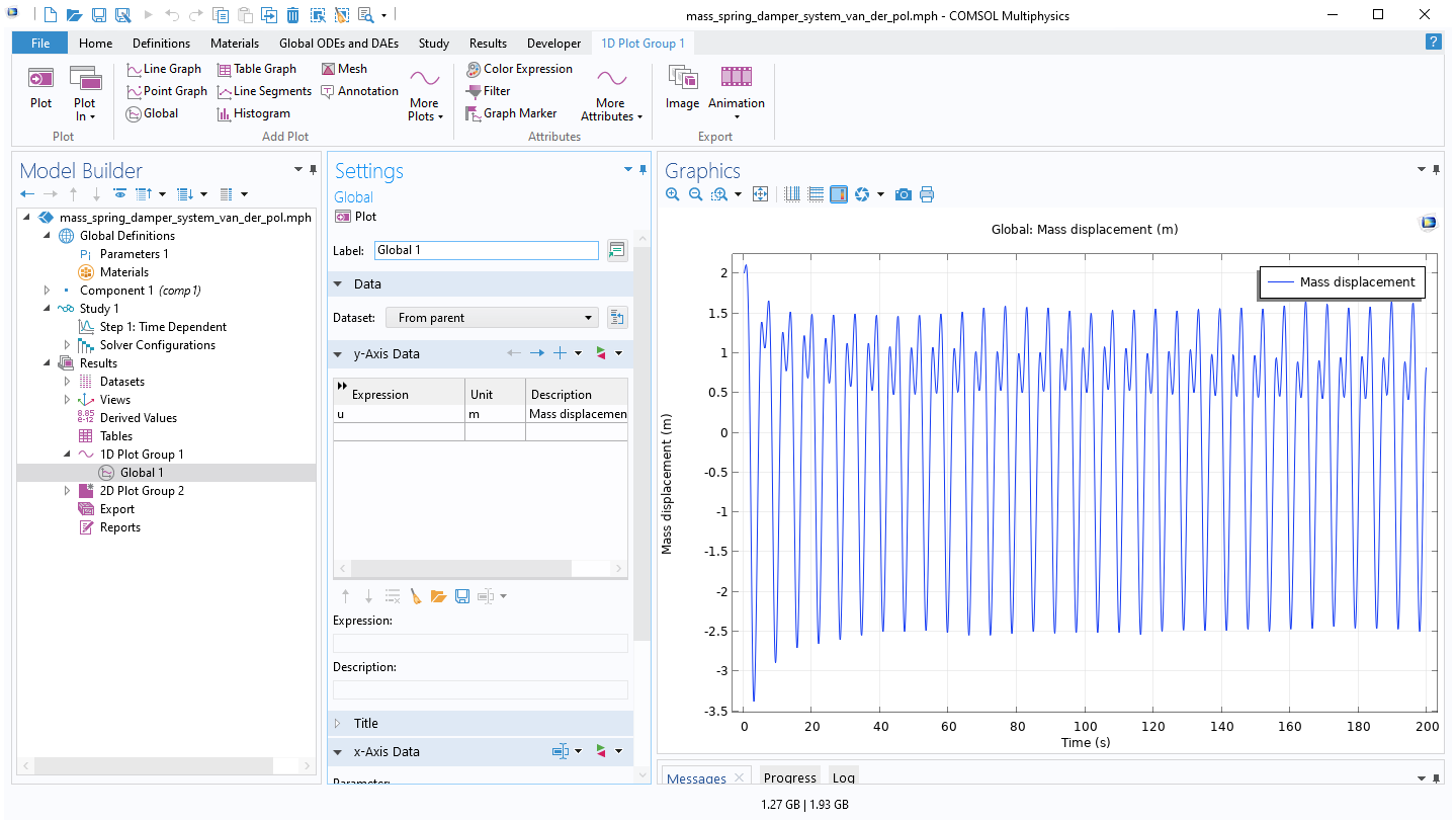 The Model Builder with the Global plot selected, the settings, and the Graphics window showing the solution.
The solution to the van der Pol oscillator differential equation.
It also gives the following phase-plane plot:
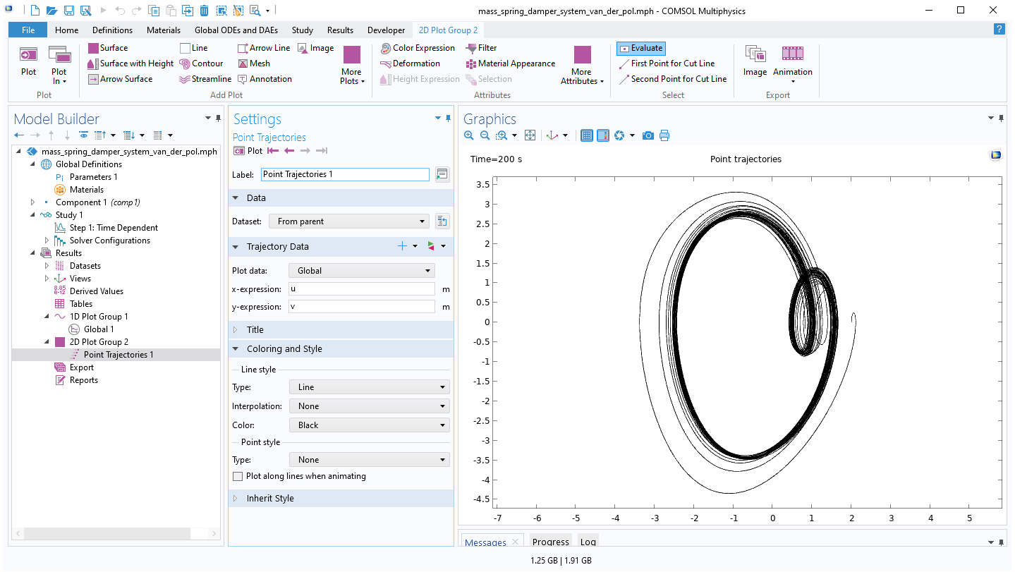 The Model Builder with the Point Trajectories plot selected, the corresponding Settings window, and the Graphics window showing the van der Pol oscillator phase plot.
The phase plot for the van der Pol oscillator differential equation.
The darker portion of this plot indicates that the solution has a so-called limit cycle. For the solution in the time domain, this is due to the fact that it approaches a limiting periodic solution. However, this limiting waveform is not sinusoidal but has a more complicated behavior. We can see its shape more clearly by zooming in on the last few cycles in the time-domain plot, as shown below:
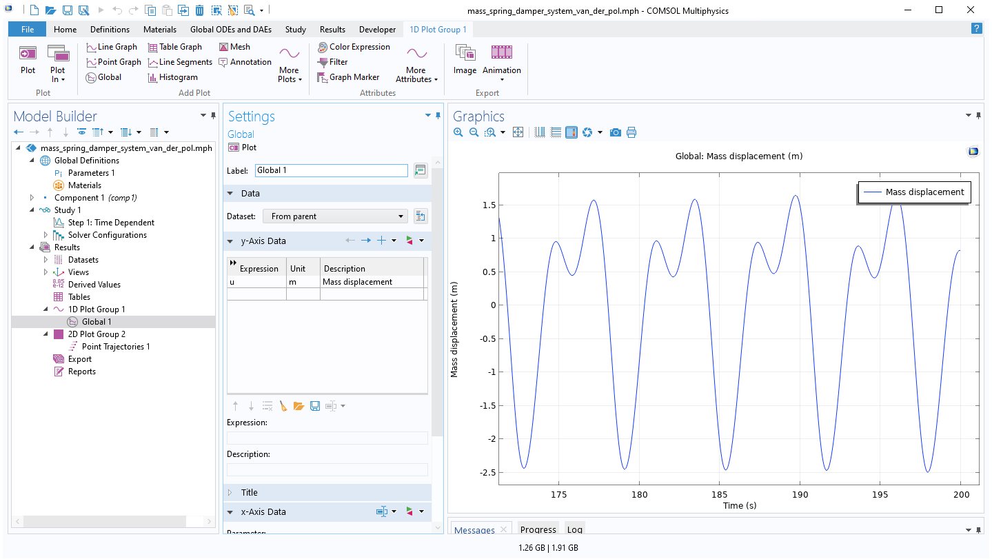 The Model Builder with the Global plot selected, the plot settings, and the Graphics window with the plot zoomed in.
A zoomed-in view of the solution to the van der Pol oscillator differential equation.
By changing the value of the damping (or gain) coefficient c, you can get other waveforms. Note that the nonlinearity of the equation also shifts the dominant frequency. The figure below shows the waveform for c=10[kg/s].
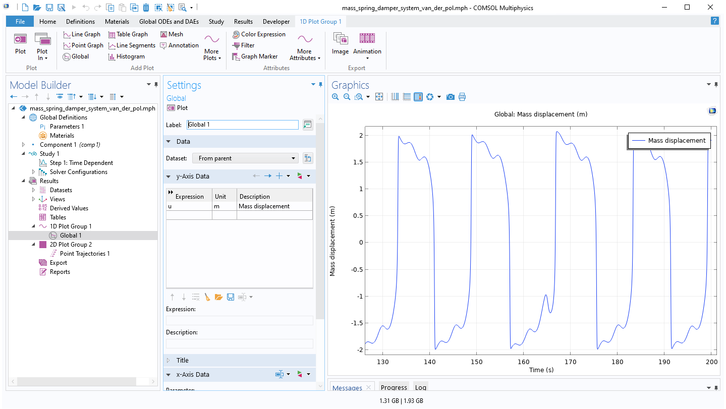 The Model Builder with the Global plot selected, the Global Settings window, and the Graphics window showing the new mass displacement waveform.
The solution to the van der Pol oscillator differential equation for a different damping coefficient.
This waveform has a much more complicated frequency spectrum than the linear mass-spring-damper system, as shown in the figure below using logarithmic scaling:
 The Model Builder with the Global plot selected, the corresponding Settings window, and the Graphics window showing the frequency spectrum become more complex.
The frequency spectrum of the solution to the van der Pol oscillator differential equation.
Plotting Phase Portraits
Many text books have illustrations of the phase portrait of the unforced van der Pol oscillator:


We get an expression that we can use to plot the phase portrait by first rearranging:


We will get the phase portrait by identifying u with the x-coordinate and v with the y-coordinate. To get the arrow plot we want, we set:
 as the x-component
and
 as the y-component
We will plot this vector field using a Grid 2D dataset with coordinates x and y instead of u and v. This means that the actual vector-field expression to use will be:
x component: y
y component: (c*(1-e*x^2)*y-k*x)/m
The figure below shows a phase portrait for c=1[kg/s] and a trajectory for the initial condition (u, v) = (-3, -3).
A phase portrait of the solution to the van der Pol oscillator.
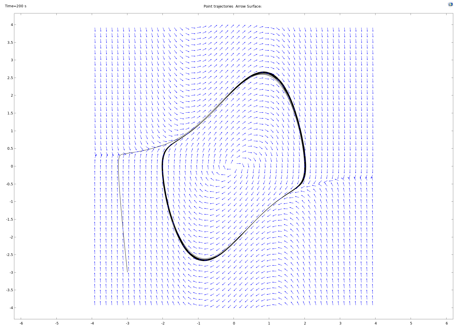 A close-up view of the phase portrait of the van der Pol oscillator solution.
Close-up of the phase portrait of the solution to the van der Pol oscillator.
The corresponding file is available in the set of downloadable files associated with this article.
Differential-Algebraic Systems
In Part 5 of this course, we described how a time-dependent Joule heating model is a form of a DEA system since one of the equations does not have time derivatives. In the same way, the Global ODEs and DAEs interface can handle DAE systems.
For example, the following system has a time derivative in the first equation, but not in the second:


The figure below shows this DAE system in the user interface:
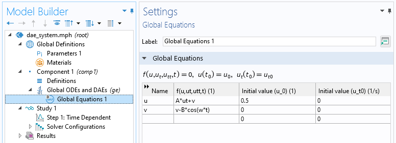
The differential algebraic equation system entered in the Global Equations interface.
Note that the Initial value for the second equation does not come into play since there is no time derivative.
The figure below shows the solution to this system:
 The Model Builder with the Global plot selected, the settings, and the Graphics window showing the state variable u in blue and the state variable v in green.
The solution to the differential algebraic equation system.
The parameters used in this example are shown in the figure below:
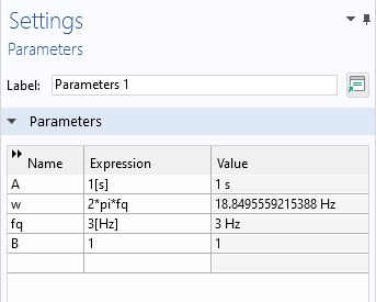
The parameters to the differential algebraic equation system.
Coupling PDE Models with ODEs
You can add one or more Global Equations interface to an existing physics interface in order to create customized couplings with ODEs. The figure below shows a Global Equations interface added to an Electric Currents interface:
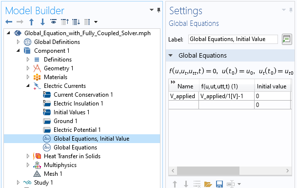
The Global Equation settings for an algebraic equation linked to the equation of an Electric Currents interface.
Coupling field variables from a physics interface with one or more ODEs is illustrated in a number of our blog posts, including:
- "Using Global Equations to Introduce Fully Coupled Goal Seeking"
- "Introducing Goal Seeking into the Segregated Solver"
- "Accelerating Model Convergence with Symbolic Differentiation"
In addition, a related topic that you should explore is state variables. For more information on this topic, see our blog post "How to Use State Variables in COMSOL Multiphysics®".
There are some important sign considerations when creating customized couplings between equations. In COMSOL Multiphysics, the convention is that an external (generalized) force acting on a system should enter the equations with a positive sign. This means that the mass-spring-damper equation should, when coupled with other equations, preferably be written as:


This sign convention does not matter as long as you are only modeling using ODEs. However, it does matter if you, for example, couple this with a solid using a Solid Mechanics interface. Such a model could be used for a mass that is glued to a surface on an elastic object. If you use the sign convention with  , you can couple using a simple bidirectional constraint. If you instead use
  , then you need to switch the sign in the constraint force expression. In the latter case, the symmetry of the coupled system will be broken, and you will end up with an equation system that has a nonsymmetric system matrix that is less efficient to solve.
The Lorenz Equation System
In the early 1960s, the Lorenz equation system was developed to model atmospheric convection. Lorenz discovered that the solution exhibited chaotic behavior for certain parameter values and initial conditions. The solution, when plotted in phase space, resembles the figure eight, as shown below. The Lorenz attractor is a set of chaotic solutions of the Lorenz system as viewed in phase space. A COMSOL Multiphysics implementation of this system, with detailed documentation, can be downloaded here.
The Lorenz system, which is nonlinear, can be written as follows:


with initial conditions:


Here, the parameters a, b, and c are generally positive scalar numbers. Not all solutions are chaotic, but Lorenz found that the values a = 10, b = 8/3, and c = 28 give a system with a chaotic behavior. The settings below show the Lorenz equation system with the following initial conditions:
u= −10v= −4.45w= 35.1
The parameter pert is used to illustrate how the system is sensitive to small changes in the initial conditions.
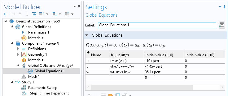
The Lorenz equation system entered in the Global Equations interface.
The figure below shows the solution between 0 s and 35 s:
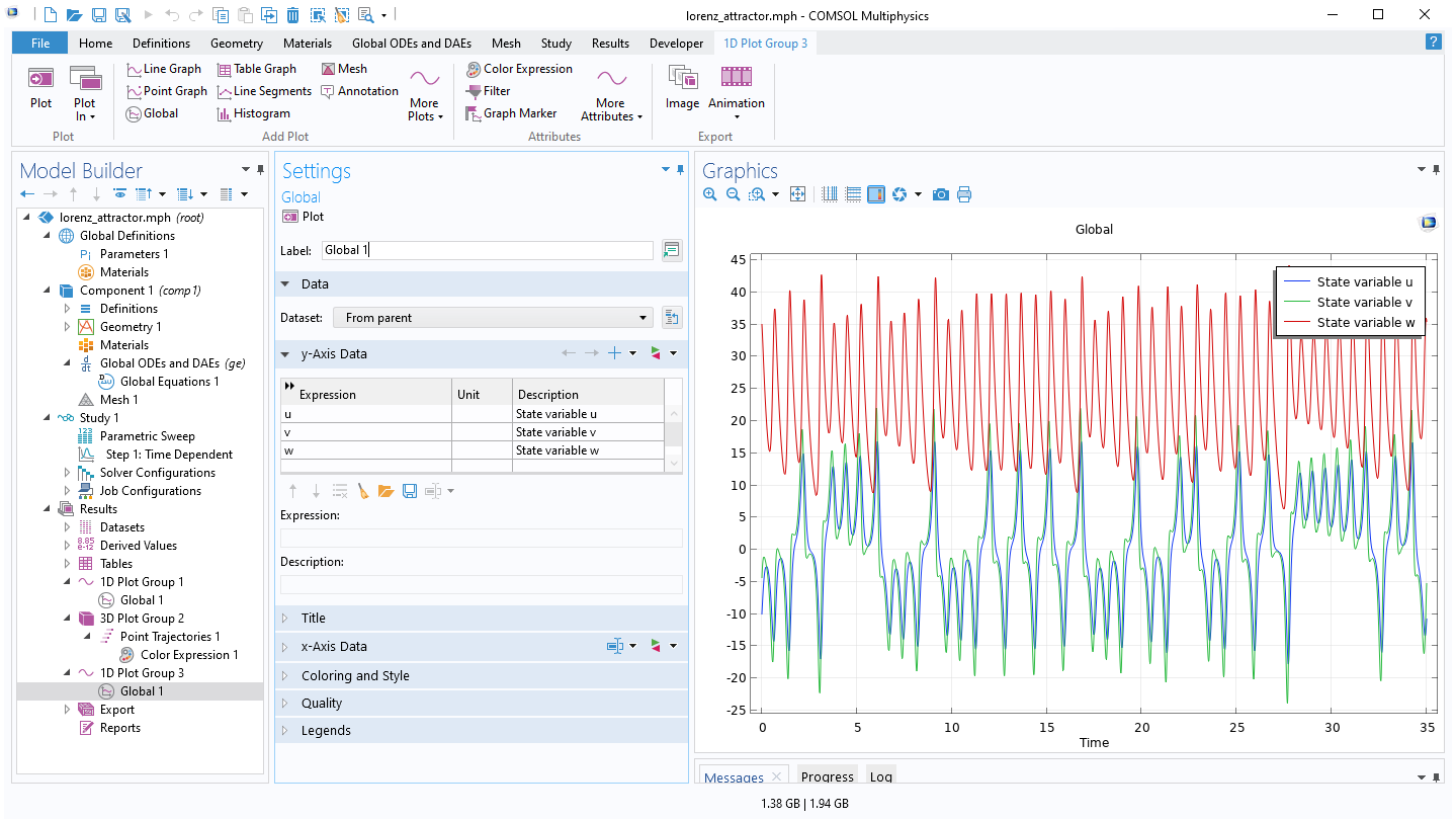 The Model Builder with the Global plot selected, the plot settings, and the Graphics window showing the state variable u in blue, the state variable v in green, and the state variable w in red.
The solution to the Lorenz equation system.
The solution in 3D phase space shows the characteristic shape of the Lorenz attractor.
 The Lorenz attractor with the outer section being red, the middle section being yellow, and the inner section being green.
The phase portrait of the Lorenz equation system showing the characteristic shape of the Lorenz attractor.
Among the files available for download with this article, you will also find a version of the van der Pol oscillator with a similar type of phase-space plot in 3D, with time (scaled) as the third axis:
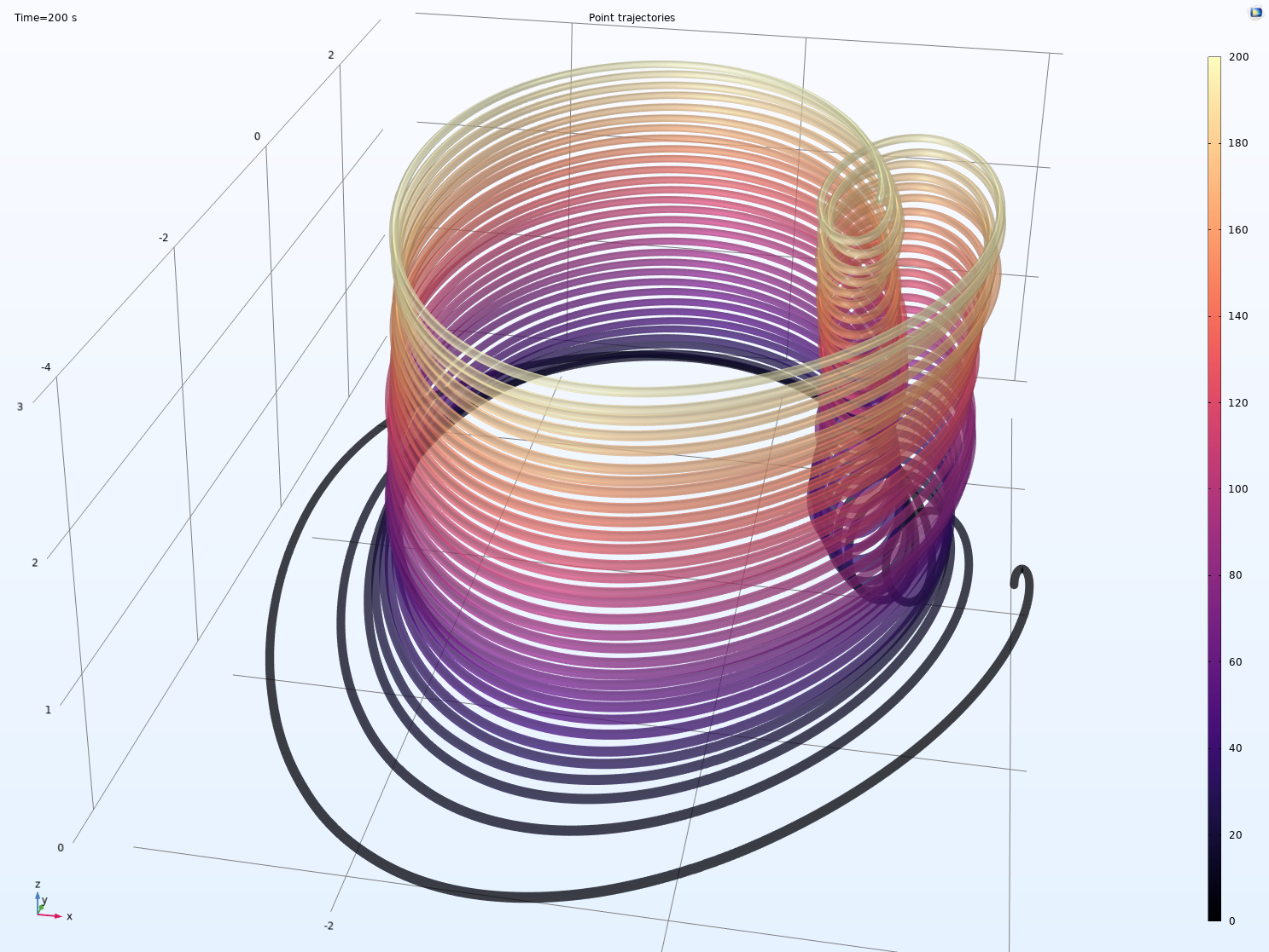 A 3D phase-space plot showing the shape in mostly purple and red, with black near the bottom and yellow near the top.
A 3D phase-space plot of the solution to the van der Pol oscillator equation.
Further Learning
Although the models used throughout this article are available for download, we encourage you to build the models yourself following the guidance provided here. This will help to reinforce how to set up ODEs in the software using the Global ODEs and DAEs interface.
このページに関するフィードバックを送信, または サポートに連絡 してください.