Manually Implementing a Boundary Terminal Condition
When using the Electric Currents interface in the AC/DC Module and the MEMS Module, the Boundary Terminal condition imposes the condition that an equipotential is applied across all selected boundaries. This applied potential can be solved for such that a specified total current is applied. This functionality can be manually reproduced as described in this article. It is also possible to extend this manual implementation and apply an excitation condition on interior boundaries.
Implementing the Boundary Terminal Condition with Fixed Current on Exterior Boundaries
To manually implement a custom condition that matches the functionality of the Boundary Terminal condition, begin with a model that uses the Electric Currents interface, such as a model of a straight cylinder of copper wire of radius 0.5[mm] and length 10[mm].
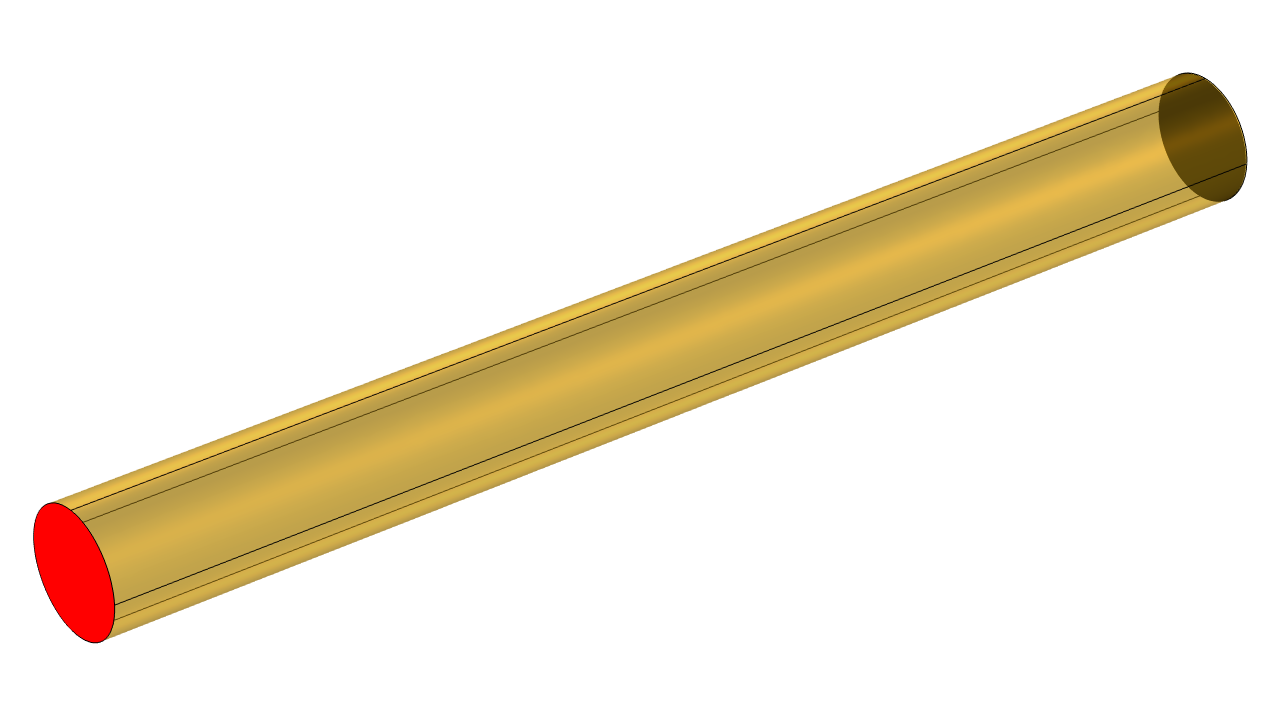 A yellow cylinder with a red circular face on one end.
A straight section of copper wire, grounded at one end, excited at the other.
A yellow cylinder with a red circular face on one end.
A straight section of copper wire, grounded at one end, excited at the other.
Apply a Ground condition at one end of the cylinder, which fixes the electric potential to zero. At the other end, apply an Electric Potential condition. To start, apply any arbitrary potential (e.g., 1 mV) and solve using a Stationary study to verify that the current flows from higher potential to lower potential. Evaluate the current flowing through the boundary using a component coupling. See the article "Computing Space and Time Integrals" for reference.
This procedure reproduces the Boundary Terminal condition of type Voltage.
To instead impose the condition that a fixed current flows through the boundary, an additional degree of freedom needs to be introduced. This is done by introducing a Global Equations feature within the Electric Currents interface. This feature should be added to the Electric Currents interface so that the software will treat it as a fully coupled variable.
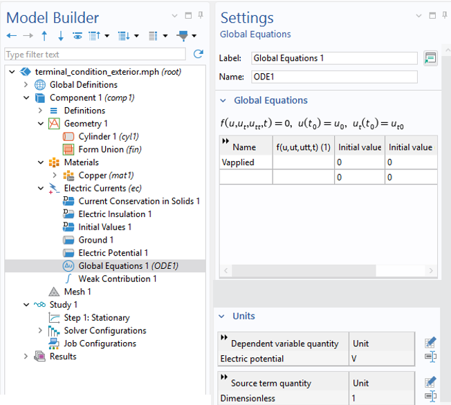 A settings window for global equations with an empty equation for Vapplied.
The settings for the Global Equations feature, showing the empty equation and the Units settings.
A settings window for global equations with an empty equation for Vapplied.
The settings for the Global Equations feature, showing the empty equation and the Units settings.
Within the Global Equations feature under the Electric Currents interface, specify a name for the additional unknown, such as Vapplied, and specify the Units to be Electric Potential. Leave the equation field empty because the load will be applied via a weak contribution. This step introduces an additional degree of freedom into the model, which is used to set the applied electric potential within the Electric Potential boundary condition.
 The electric potential is defined by the Vapplied.
The additional unknown is the applied electric potential.
The electric potential is defined by the Vapplied.
The additional unknown is the applied electric potential.
At this point, an additional degree of freedom has been added to the model, but no condition has been given regarding this degree of freedom. The automatic constraint handling imposes the condition that no net current flux is imposed at these boundaries and that the electric potential is uniform. That is, the integral of the current equals zero.
To impose instead the condition that a specified total current flows into the model, a Weak Contribution feature is added, with the expression:
test(Vapplied)*1[A]
The desired current, here 1 Amp, is applied as a load to the unknown, Vapplied, and the automatic constraint handling distributes this load over the entire boundary, while simultaneously imposing the condition that the surface is at an equipotential. It is also possible to specify the current via a Global Parameter or a Variable that changes over time, rather than a numerical constant.
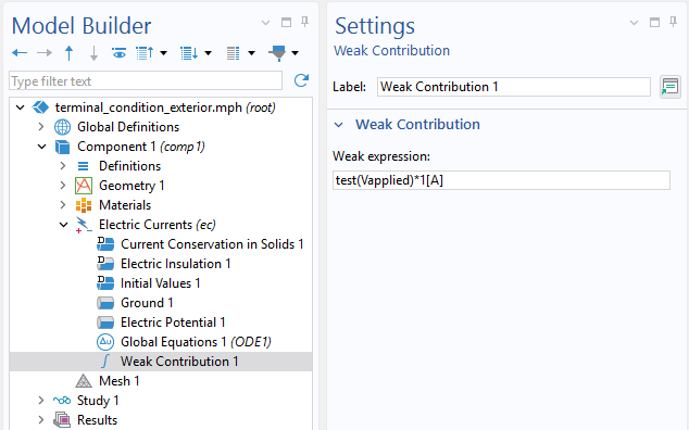 The weak contribution expression entered in the settings window.
The Weak Contribution feature applies a load to the degree of freedom, the applied electric potential.
The weak contribution expression entered in the settings window.
The Weak Contribution feature applies a load to the degree of freedom, the applied electric potential.
Solve and observe that the number of degrees of freedom has increased by one, as compared to the original model. Evaluate the integral of the current through the boundary, as well as the unknown, Vapplied.
This completes the manual implementation of the current-controlled Boundary Terminal condition. The model can be compared to the Application Gallery example Computing the Resistance of a Wire.
Implementing on Interior Boundaries
It is sometimes desired to solve for the currents within a closed loop, without a beginning or end. An example model of a closed loop in the shape of a torus is available for download and is pictured below.
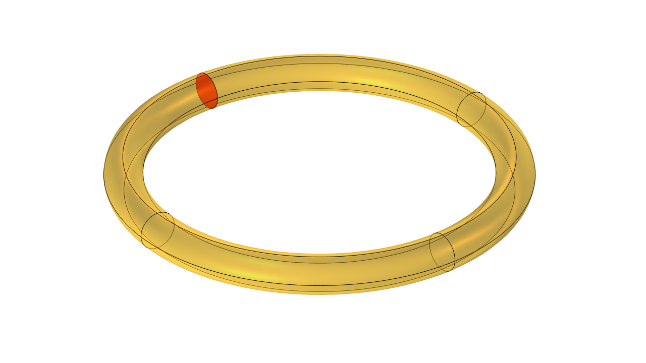 A yellow toroidal loop with a single red circular interior boundary.
A toroidal loop of copper with an interior slit boundary that bisects the cross-section.
A yellow toroidal loop with a single red circular interior boundary.
A toroidal loop of copper with an interior slit boundary that bisects the cross-section.
To begin, introduce an interior boundary to the geometry that cuts through the entire cross-section and is as perpendicular as possible to the expected direction of current flow. For a torus, this can be done by first adding a Work Plane through the centerline.
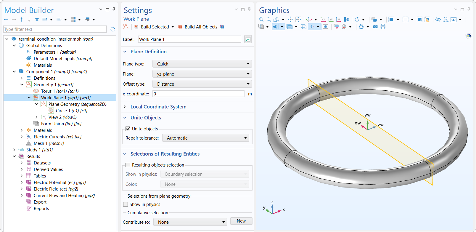 A yellow plane passes through the central axis and a gray toroidal loop.
An example of a Work Plane feature that passes through the centerline.
A yellow plane passes through the central axis and a gray toroidal loop.
An example of a Work Plane feature that passes through the centerline.
Then, in this case, a circle was used to create the internal boundary in the Plane Geometry feature.
 A 2D sketch of the cross section of a loop with a blue circle on the left, and a gray circle on the right.
An example of how a boundary can be created, in this case by creating a Circle on the Plane Geometry.
A 2D sketch of the cross section of a loop with a blue circle on the left, and a gray circle on the right.
An example of how a boundary can be created, in this case by creating a Circle on the Plane Geometry.
Add an Auxiliary Slit feature and apply it to the interior boundary to represent a split, or discontinuity, in the electric potential field, which by default is called V. This feature duplicates the degrees of freedom on the selected boundary and allows the potential field to be different on the upside and downside, representing a jump in the potential field across an idealized zero-thickness source. These different values are addressed via the up() and down() operators. This slit must entirely bisect the volume through which the current flows.
Two Constraint features are used to impose conditions at this slit. The first Constraint expression is:
down(V)
This imposes the condition that the electric potential on the downside is zero and is equivalent to the Ground condition. The second constraint expression is:
up(V)-Vapplied
This sets the potential on the upside equal to Vapplied. Note that the upside/downside is, in general, arbitrary, so these can be reversed if desired.
Next, repeat the addition of the Global Equation for Vapplied and the Weak Contribution. This step is identical to the exterior boundary case.
The solution shows that the electric potential field has a jump across the slit boundary. The current flows in a continuous loop through the coil. The source is approximated as being at the interior boundary, that is, a battery that has zero thickness.
 A toroidal loop on the left is colored on the surface with a rainbow gradient and a toroidal loop on the right has arrows inside it.
The electric potential (left) has a discontinuity at the slit. The current flow (right) is smooth around the closed conductive loop.
A toroidal loop on the left is colored on the surface with a rainbow gradient and a toroidal loop on the right has arrows inside it.
The electric potential (left) has a discontinuity at the slit. The current flow (right) is smooth around the closed conductive loop.
このページに関するフィードバックを送信, または サポートに連絡 してください.