Using Uncertainty Quantification to Model Frequency Variation in a MEMS Resonator
Uncertainty quantification (UQ) can significantly enhance finite element method (FEM) analysis of microelectromechanical systems (MEMS). It can predict the uncertainty of a functional parameter resulting from variation in the fabrication process. This can then be used to:
- Evaluate the manufacturability of a design
- Set process control goals for manufacturing
When using COMSOL Multiphysics® with the MEMS Module and the Uncertainty Quantification Module, there are several study types available for analyzing the uncertainty of a quantity of interest (QoI) based on the variation of input parameters. In this article, we will discuss how to use these studies, using a model of a MEMS resonator as an example.
Background: MEMS Resonators and Manufacturing Variation
The solidly mounted resonator (SMR) is a type of bulk acoustic wave resonator commonly used as a bandpass filter in communication systems. SMRs operate in the GHz frequency range, are relatively easy to manufacture, and have low loss. In an SMR, a piezoelectric layer is made to vibrate in the so-called thickness-extension mode between two electrodes — the electric field causes it to expand and contract in the vertical direction.
The SMR in this tutorial model is fabricated on a substrate by first depositing alternating layers of silicon dioxide (SiO2) and molybdenum (Mo). Next, an aluminum (Al) layer is formed as the bottom electrode, followed by deposition of a zinc oxide (ZnO) piezoelectric layer. Finally, an Al top electrode is deposited. The nominal layer thicknesses are shown in Figure 1.

Figure 1. A cross section of the SMR showing the substrate, SiO2, Mo, Al, and ZnO layers, together with a surface plot of the elastic energy showing confinement at the center of the piezoelectric layer.
The various layers are formed by physical vapor deposition, and each layer's thickness has a variation that introduces uncertainty to the operating frequency of the SMR. Following the tutorial model of a solidly mounted resonator in 2D, we assume that each layer's thickness varies according to a normal distribution, defined by its values for mean thickness and standard deviation. Details of the operation of this tutorial model can be found in the corresponding documentation in the Application Libraries. In this article, the focus is on how to specify the statistical variation of the layer thicknesses and how to compute the uncertainty in the SMR's operating frequency,  .
.
Input Parameters and Quantities of Interest
In the process of conducting a UQ study, a series of QoIs are identified that are derived from the solution. These quantities depend on the input variables. Any uncertain input, whether related to a physical scenario, a geometric dimension, a property of materials, or a discretization approach, is considered an input parameter. These parameters can be assigned probabilities through analytical sampling or specified directly by the user. When sampled analytically, the inputs may exhibit correlation or independence, with correlated parameters being organized into groups for sampling via the Gaussian copula technique. A QoI can be any global quantity that is solution dependent. For instance, in structural analysis, such quantities could include the peak displacement, stress levels, or angle of deflection. In heat transfer or CFD, they might represent the maximum temperature, overall heat loss, or total fluid-flow rate.
For the MEMS resonator demonstrated in this article, the layer thickness values are used as input parameters and the operating frequency is used as the QoI.
Selecting the Correct Resonance Frequency as the QoI
The SMR's operating frequency, , corresponds to the thickness-extension mode, where vibrational energy is confined to the center of the piezoelectric layer, as shown in Figure 1. The unique symmetry of the displacement field is the natural result of the symmetry of the applied electric field, and any other modes could never be excited. When using the Eigenfrequency study, however, the settings required to find of the thickness-extension mode will also return other solutions in its proximity. For example, Figure 2 shows the plots of the displacement field for various eigenmodes that are returned by the Eigenfrequency study. Other than , these are the so-called spurious modes and are of no interest. Moreover, because UQ requires the QoI to be a single-valued, real quantity, the UQ study needs to automatically select only through some enforceable criteria.
 |
 |
 |
|---|---|---|
| = 870.54 MHz |
 = 870.94 MHz = 870.94 MHz |
 = 871.61 MHz = 871.61 MHz |
 |
 |
 |
 = 873.75 MHz = 873.75 MHz |
 = 875.20 MHz = 875.20 MHz |
 = 876.92 MHz = 876.92 MHz |
Figure 2. Surface plots of the y-displacement of some of the solutions of the eigenfrequency study. The only "correct" (nonspurious) eigenmode for this problem is the thickness-extension mode vibrating at 870.54 MHz.

Figure 3. The surface plot of y-displacement, or  , shows deformation of the top electrode. The absolute value of displacement along the width of the top electrode can be used as a criterion for selecting the eigenfrequency solution associated with the thickness-extension mode.
Taking a closer look at the thickness-extension mode in Figure 3, we can see the symmetry of the deformation of the piezoelectric layer below the top electrode. We can define the quantity displacement phase uniformity, or  , as:
, as:

where is the y-displacement and the integration limits  and
and  are the boundaries of the top electrode. Plotting versus eigenfrequency generates the plot in Figure 4.

Figure 4. A plot of versus eigenfrequency for the nominal values of input parameters, showing 30 returned solutions. At = 870.54 MHz, = 1, while for other solutions, << 1.
Figure 4 shows that = 870.54 MHz is unique for having = 1 while other solutions have << 1. We can discard the unwanted modes after the Eigenfrequency study step by using the Combine Solutions study step and selecting the Remove solutions setting along with the other settings shown in Figure 5, with the condition expressed as:
Excluded if: abs(comp1.intop1(comp1.v))/(comp1.intop1(abs(comp1.v)))<0.99.
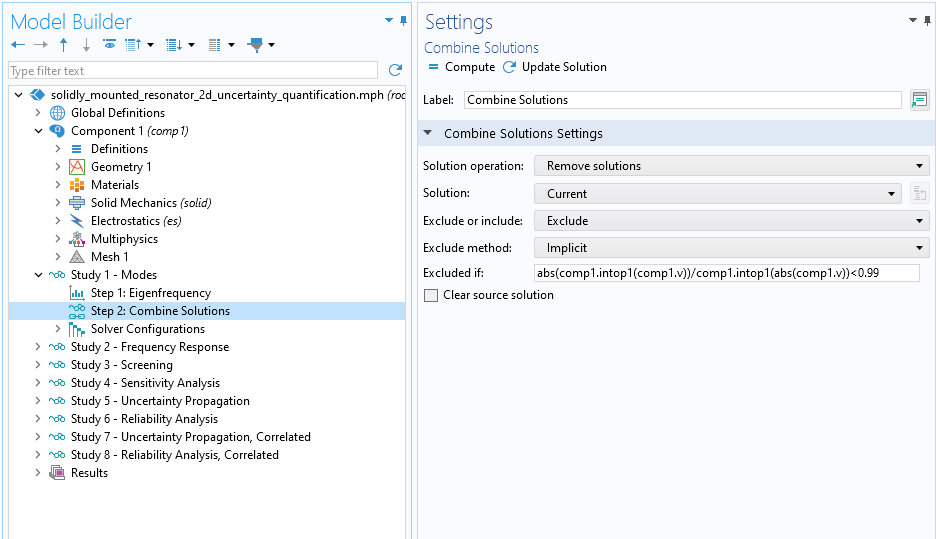 The Model Builder with the Combine Solutions node selected and the corresponding Settings window showing the settings for excluding spurious modes.
Figure 5. The settings to exclude the unwanted spurious modes.
Now, we can use the Eigenfrequency study step as the reference study for UQ. For the QoI, we simply use the single-valued solution of the Eigenfrequency study.
The Uncertainty Quantification Studies
The Uncertainty Quantification Module provides five different study types: Screening, Sensitivity Analysis, Uncertainty Propagation, Reliability Analysis, and Inverse Uncertainty Quantification.
Following is a quick summary of each UQ study type:
- Screening:
- Identifies the most influential inputs for each QoI
- Based on the Morris one-at-a-time (MOAT) method
- Outputs MOAT mean and MOAT standard deviation values
- Sensitivity Analysis:
- Computes the fraction of impact for the inputs for each QoI
- Outputs first-order and total Sobol indices
- Uncertainty Propagation:
- Computes the statistical variation of a quantity of interest
- Outputs a kernel density estimation (KDE) plot representing an estimate of the probability distribution of the QoI
- Reliability Analysis:
- Computes the probability for the fulfillment of a condition based on a QoI, e.g., "What is the probability that a certain quantity exceeds a threshold?"
- Inverse Uncertainty Quantification:
- Uses experimental data to backtrack and uncover the statistical properties of certain input parameters, starting with some initial assumptions about them (prior probability distribution)
- Applies surrogate models and statistical methods to refine the characterization of these inputs, providing (posterior) probability distributions, as well as a confidence interval table containing the mean, standard deviation, min/max values, and confidence bounds
To extract statistical data from a physics model, you need to run many simulations via a Monte Carlo method, varying the parameters of the inputs according to their probability distributions. For a 3D model, directly applying a Monte Carlo method might be computationally infeasible. To circumvent this, the Uncertainty Quantification Module first builds up a so-called surrogate model that is used for sensitivity analysis, uncertainty propagation, reliability analysis, and inverse UQ, but not for screening.
The first four study types are demonstrated below using the solidly mounted resonator in 2D tutorial model. We will review these study types further and see how they are applied to the MEMS resonator model.
The Screening Study
The Screening, MOAT study implements a lightweight global screening method that provides a qualitative measure of the importance of each input parameter. The method is purely sample based, using the Morris one-at-a-time (MOAT) method, and requires a relatively small number of COMSOL model evaluations. This makes it an ideal method when the number of input parameters is too great to allow more computationally expensive UQ studies.
Figure 6 illustrates the type of sampling used by the MOAT method for three input parameters:  ,
,  , and
, and  .
.

Figure 6: An illustration of the MOAT method where the value for each input variable is changed by a predetermined step while keeping the other input variables constant.
First, the range for each parameter is specified. Then, a starting point is chosen by picking a set of random input parameters  . For each input variable, its value is now changed by a predetermined step while keeping the other variables constant. Finally, the change in output induced by this elementary effect is observed. This is repeated until there is a sufficient number of samples to obtain reliable information about each parameter's effect. As a general rule, if the number of input parameters is
  , then the number of model evaluations would be
  . In the example above, we would choose
  .
.
For each QoI, this MOAT method computes the MOAT mean and MOAT standard deviation for each input parameter. These values are presented in a MOAT scatter diagram, as shown for the MEMS resonator in Figure 9 below. The ranking of the MOAT mean and MOAT standard deviations indicates the relative importance of the input parameters. A high MOAT mean value implies that the parameter is significantly influencing the QoI. A high MOAT standard deviation value implies that the parameter is influential and that it is either strongly interacting with other parameters, has a nonlinear influence, or both.
Screening Applied to the MEMS Resonator
Let's now apply the Screening, MOAT study to identify the most influential inputs for each QoI in the MEMS resonator model. Recall that the input parameters are the thickness values of the SiO2, Mo, Al, and ZnO layers and that they contribute to the uncertainty in resonant frequency. To save computation time, a screening study can be used to identify the input parameters with the least impact and then exclude these from subsequent studies. Since we already have an Eigenfrequency study step in our model (Study 1), we can use it as a reference study for the Screening, MOAT study. This means the eigenfrequency will be solved for various combinations of input parameter values generated by the screening study. To set up the screening study, we right-click the Study 1 node and, under Uncertainty Quantification, choose Add Uncertainty Quantification Study Using Study Reference. The newly generated study will have the screening study type selected automatically. In the Settings window of the study, enter the expression real(freq) in the table for Quantities of Interest. The real() operator ensures that we only consider the real part of the otherwise complex-valued frequency. Due to numerical errors, there will always be a small imaginary part. Note that if the model includes damping, there will be a larger imaginary part.

Figure 7. The settings to specify eigenfrequency as the QoI.
In the table for Input Parameters, specify t_pe (Piezoelectric layer thickness) for ZnO, t_lil (Low impedance layer thickness) for Mo, t_hil (High impedance layer thickness) for SiO2, and t_pe (Electrode thickness) for Al.

Figure 8. The settings to specify the film thicknesses as input parameters.
Computing the screening study results in the MOAT plot in Figure 9, which shows that the thickness of the high impedance layer has an insignificant effect and can be removed from subsequent studies.

Figure 9. A plot of the MOAT mean and MOAT standard deviation values from the Screening, MOAT study.
Sensitivity Analysis
The Sensitivity Analysis study type is used to determine the responsiveness of specific QoIs in relation to variations in input parameters. It includes two different approaches: the Sobol and correlation methods.
For the Sobol method, the analysis covers the full distribution of input parameters, breaking down the variance observed in each QoI into segments resulting from the inputs and their mutual interactions. Through the Sobol method, two so-called Sobol indices for each input parameter are calculated: These are the first-order Sobol index and the total Sobol index.

Figure 10: First-order and total Sobol indices for a sensitivity analysis (of a different model, not the MEMS resonator model.)
The first-order Sobol index quantifies how much of the variance in a QoI can be ascribed to changes in each input parameter on its own. Meanwhile, the total Sobol index accounts for the variance in a QoI due to both individual input parameter variances and their combined effects. A specialized Sobol plot, the Sobol Index plot, is used to visualize these indices, arranging histograms according to the total Sobol index. The parameter that yields the highest total Sobol index is deemed the most influential on the QoI. The disparity between the total and first-order Sobol indices for a parameter indicates the magnitude of its interactions with other parameters.
Compared to the screening method, which is largely qualitative, sensitivity analysis is used to quantitatively analyze how uncertainties in the QoIs apportion to the different input parameters. This method requires more computational resources since the computation of accurate Sobol indices relies on a high-quality surrogate model.
The correlation technique, not demonstrated here, identifies both linear and nonlinear correlations between the QoIs and each input parameter. When employing this method for sensitivity analysis, it calculates four varieties of correlations: bivariate, ranked bivariate, partial, and ranked partial, to establish how input parameters linearly or monotonically relate to the QoIs. To analyze the MEMS resonator, only the Sobol method will be used.
Sensitivity Analysis Applied to the MEMS Resonator
In the previous study, we determined that the SiO2, Al, and ZnO layer thicknesses were important enough to warrant further study. As a next step, we will use a Sensitivity Analysis study to better quantify the relative importance of each layer's varying thickness. When setting up the Sensitivity Analysis study, we use the screening study as a reference by selecting Add New Uncertainty Quantification Study For and then choosing Sensitivity Analysis. The sensitivity analysis will inherit the settings of the Screening study. After computing the result, the Sobol indices plot is generated (Figure 12).
 The Model Builder with the Uncertainty Quantification node selected and its corresponding menu showing the option to add a new UQ study for a sensitivity analysis.
Figure 11. Adding a new Sensitivity Analysis study.

Figure 12. First-order and total Sobol indices for the MEMS resonator sensitivity analysis.
Uncertainty Propagation
The Uncertainty Propagation study type is designed to examine the effect of input parameters' uncertainties on each QoI by estimating their probability density functions (PDFs). The potentially complex relationships between input parameters and QoI, obtained via COMSOL Multiphysics model evaluations, are typically beyond the scope of direct analytical solutions for most scenarios.
Due to this complexity, Monte Carlo simulations are used to estimate the PDFs. Similar to the approach used in the Sobol method, surrogate modeling is applied to significantly decrease the computational demands of the Monte Carlo simulations. For each QoI, a kernel density estimation (KDE) is carried out to closely approximate its PDF, which is then represented graphically. This analysis also generates a confidence interval table. This table details, for every QoI, important statistical measures such as the mean, standard deviation, and the minimum and maximum values. It also includes the lower and upper boundary values at confidence levels of 90%, 95%, and 99%.

Figure 13: An illustration of how the probability distribution of input parameters results in a probability distribution of a QoI (output parameter). The heights of the graphs represent the probability density of a certain value of the input or output. The distribution of the QoI represents the combined effect of all input parameters.
Uncertainty Propagation Applied to the MEMS Resonator
Now we can compute the distribution of the QoIs and the resonant frequency resulting from the thickness variation of the SiO2, Al, and ZnO layers. To set up the Uncertainty Propagation study, use the Sensitivity Analysis study as a reference; choose Add New Uncertainty Quantification Study For and then select Uncertainty Propagation to keep the same settings so you don't have to specify the Quantities of Interest or Input Parameters again. Computing the study generates the KDE plot shown in Figure 14. This plot shows an estimate of which resonant frequency values are most likely to occur considering variations in layer thicknesses.

Figure 14. The Kernel density estimation for resonant frequency.
Reliability Analysis
In contrast to other types of UQ studies that focus on the overall uncertainty of the QoIs, the Reliability Analysis study uses the efficient global reliability analysis (EGRA) method to address a more specific question: Given a nominal design and a set of uncertain inputs, how likely is it that a design will fail? Failure in such a scenario is defined not only as a complete breakdown; it can also be interpreted as not meeting specific quality standards.

Figure 15: The results of a reliability analysis (of a different model, not the MEMS resonator). The contour lines for two QoIs, q1 (blue) and q2 (purple) are shown. The contour levels represent the thresholds used in the reliability analysis, q1 = 21 and q2 = 9.95. Here, two input parameters are used for illustration purposes (i.e., the x- and y-axis data). The shaded region represents the input parameter values that satisfy the reliability criteria defined by q1 < 21 and q2 > 9.95.
Traditionally, to guarantee design reliability, modeling and simulation has relied on safety margins and planning for worst-case scenarios. However, a well-conducted reliability analysis allows for a more nuanced approach, enabling precise estimations of failure probabilities, thereby avoiding both overestimations and underestimations of reliability. Preliminary estimates of reliability might be inferred from confidence intervals tied to each QoI derived from UQ studies. The EGRA method is used to delineate the boundary between failure and success in the design and gives more precise reliability criteria that take into account various combinations of QoIs and their associated thresholds.
Reliability Analysis Applied to the MEMS Resonator
In a final step, a Reliability Analysis study is added to the MEMS resonator model to calculate the likelihood of the resonant frequency being below a set lower limit of the QoI. In this case, the limit is 865 MHz, as required by overall system design. The result of the study is that the probability of not meeting this design criterion is about 3%, which provides additional data for considering redesign or setting new process control targets to reduce the layer thickness variation. The study also includes features that generate a Response Surface plot (Figure 16) that provides insights that be used to evaluate the quality of the surrogate models used in the UQ studies. The surface plot is used to visualize the relationship between the QoI, the resonant frequency, and the two most important input parameters: the thicknesses of the piezoelectric and SiO2 layers.

Figure 16. The response surface for the resonant frequency over the piezoelectric (ZnO) and silicon dioxide (SiO2) layers' thicknesses.
Further Learning
This tutorial has demonstrated how UQ is used to connect process variation to a characteristic of a device. It can be used to optimize designs by including process variation or to improve manufacturing processes. To learn more about simulating solidly mounted resonators and the Uncertainty Quantification Module, the following resources are recommended:
Note that these models require the Uncertainty Quantification Module. Additional products may also be needed; however, if you have a license for the Uncertainty Quantification Module, you can inspect all of the settings in the Model Builder.
このページに関するフィードバックを送信, または サポートに連絡 してください.