ラーニングセンター

Using FEM to Model Speaker-Room Performance

---

After a speaker driver is designed, the next step is usually to assess its performance in a real-world environment. This evaluation often considers factors such as the impact of the mounting system and the speaker's interaction with surrounding reflective, scattering, and absorbing surfaces, as well as its integration with receiving microphones, particularly in smart system design. These elements play a key role in determining the speaker's acoustic performance and ability to fuse within the broader system. In addition to sound distribution and room acoustics metrics (for indoor problems), the desired outcomes of such analyses typically include the broadband frequency response or impulse response at specific listening locations. Achieving these outcomes often necessitates combining various numerical methods and applying them in the most effective contexts, which enables precise assessments and optimizations of the acoustic environment. These simulations can also be used to generate realistic synthetic data, helping train AI models in smart devices to better handle diverse acoustic conditions without relying solely on extensive physical measurements. This multifaceted approach ensures that the analysis accurately reflects the complexities of sound behavior in different spaces.

The following numerical methods are available for modeling a speaker's behavior in a working environment. The first three methods are based on full-wave analysis, while the last method simplifies sound propagation by representing sound waves as rays:

1. Finite Element Method (FEM): This method is suitable for all types of studies across all space dimensions. This method is the most widely used method for smaller models and low-frequency analyses, where capturing the modal behavior of the environment is essential. It is especially recommended for indoor applications, particularly in scenarios involving resonant frequencies.
2. Boundary Element Method (BEM): Available for frequency-domain pressure acoustics analysis in 2D and 3D, BEM is particularly effective for scattering and reflection problems, especially when reflecting surfaces are far from the source, as meshing large fluid volumes can make FEM impractical. In speaker applications, a BEM-FEM hybrid analysis is highly useful for outdoor problems as seen in the model Vibroacoustic Loudspeaker Simulation: Multiphysics with BEM-FEM.
3. Discontinuous Galerkin Method (dG or dG-FEM): This method employs a time-explicit solver, making it memory-efficient and ideal for large transient acoustic problem. A common application is modeling the transient propagation of audio pulses in a room such as in the Wave-Based Time-Domain Room Acoustics with Frequency-Dependent Impedance model.
4. Ray Tracing: The Ray Acoustics feature, based on the ray tracing technique, is used to obtain the acoustic response in the high-frequency limit. When frequencies exceed the Schroeder frequency and full-wave approaches are computationally prohibitive or impractical, this method is often preferred.

Next, let's explore how to combine the precision of full-wave simulations with the efficiency of ray tracing to obtain a broadband frequency response. We'll focus on a speaker radiating into a furnished 5 by 4 by 2.6 meter room. We are using this simplified model to illustrate the methodology, but it is applicable to models that more accurately represent a real environment. For this type of indoor analysis, FEM is the best option for low-frequency simulations, which will be covered in this part. We'll then transition to ray tracing for higher frequencies in the following parts.

A cube with two transparent sides and geometry representing furniture inside. The geometry of the indoor room includes a suspended ceiling made of porous material backed by an air cavity, a carpeted floor, a flat-screen TV, a sideboard, a speaker, a coffee table, and a couch. A small sphere positioned above the couch represents a receiver (microphone).

Let’s now set up the FEM model for low-frequency acoustics in this room. The speaker can be modeled either with a detailed electro-vibroacoustic approach (as covered in the "Modeling Speaker Drivers in COMSOL Multiphysics^®" course) or with a lumped driver representation coupled to a FEM acoustic domain (as discussed in "Modeling Speaker Drivers – Lumped Methods").

In this example, we use a lumped circuit model for the driver, coupled to the FEM room acoustics model to capture the interaction between the speaker and the room. When applicable, this is the recommended way for modeling a speaker in a larger system (in this case, a large room) to reduce the model size. By using this approach, the acoustic characteristics of the room and the speaker’s behavior can be approximated without simulating every physical detail of the driver, significantly lowering computational complexity. The model can focus on key parameters such as frequency response, directivity patterns, and energy dispersion, enabling efficient integration with other components like room reverberation, audience absorption, and signal processing algorithms.

Moreover, this method allows rapid experimentation and optimization of speaker placement, orientation, and system tuning, all while preserving realistic acoustic performance. This approach also facilitates scalability, making it practical for complex setups where multiple speakers and interactions must be considered without a prohibitive increase in computational resources. The parameters used to describe the lumped circuit model can either come from measurement or be extracted from detailed finite element models (as discussed in "Calculating the Small-Signal Parameters of a Speaker Driver from FEA").

The FEM Room Acoustics Model

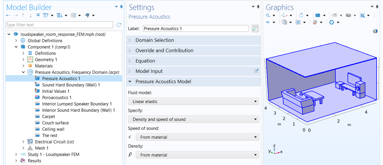
The FEM analysis uses the Pressure Acoustics, Frequency Domain physics interface to solve the acoustics in the room, in the suspended ceiling (a 1-cm thick porous layer suspended 2-cm away from the actual ceiling) and the air gap between the porous layer and the structural ceiling, as well as in the back volume of the speaker. Aside from the suspended ceiling, all other air domains are modeled using the default Linear Elastic fluid model within the Pressure Acoustics 1 material node, meaning no damping effects are included. 

An interface for pressure acoustics is selected next to a room and the interior furniture in blue. Pure air domains are modeled as lossless compressible fluid using the default settings.

The Suspended Ceiling

Sound absorption in the suspended ceiling, composed of a porous layer of fiberglass wool with a flow resistivity of 20×10³ Pa·s/m², is captured by the Poroacoustics feature. This domain feature defines equivalent fluid models to simulate sound propagation and attenuation in porous materials. These models, applicable for specific material parameters, incorporate losses in a homogenized manner and are computationally less demanding than the full Poroelastic Material model based on Biot’s theory. In this case, the simplest Delany-Bazley-Miki model, using the Miki's parameters, is selected, requiring only the flow resistivity as input. This model is specifically suitable for materials like glass and rock wool, with flow resistivity ranging between 10³ and 50×10³ Pa·s/m².

The ceiling of a room is blue, while the rest of the room is shown in wireframe. The suspended ceiling is modeled using a Poroacoustics fluid model to include damping in the porous material in a homogenized way.

The Speaker

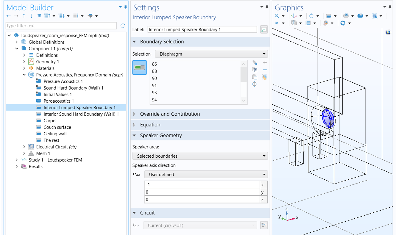
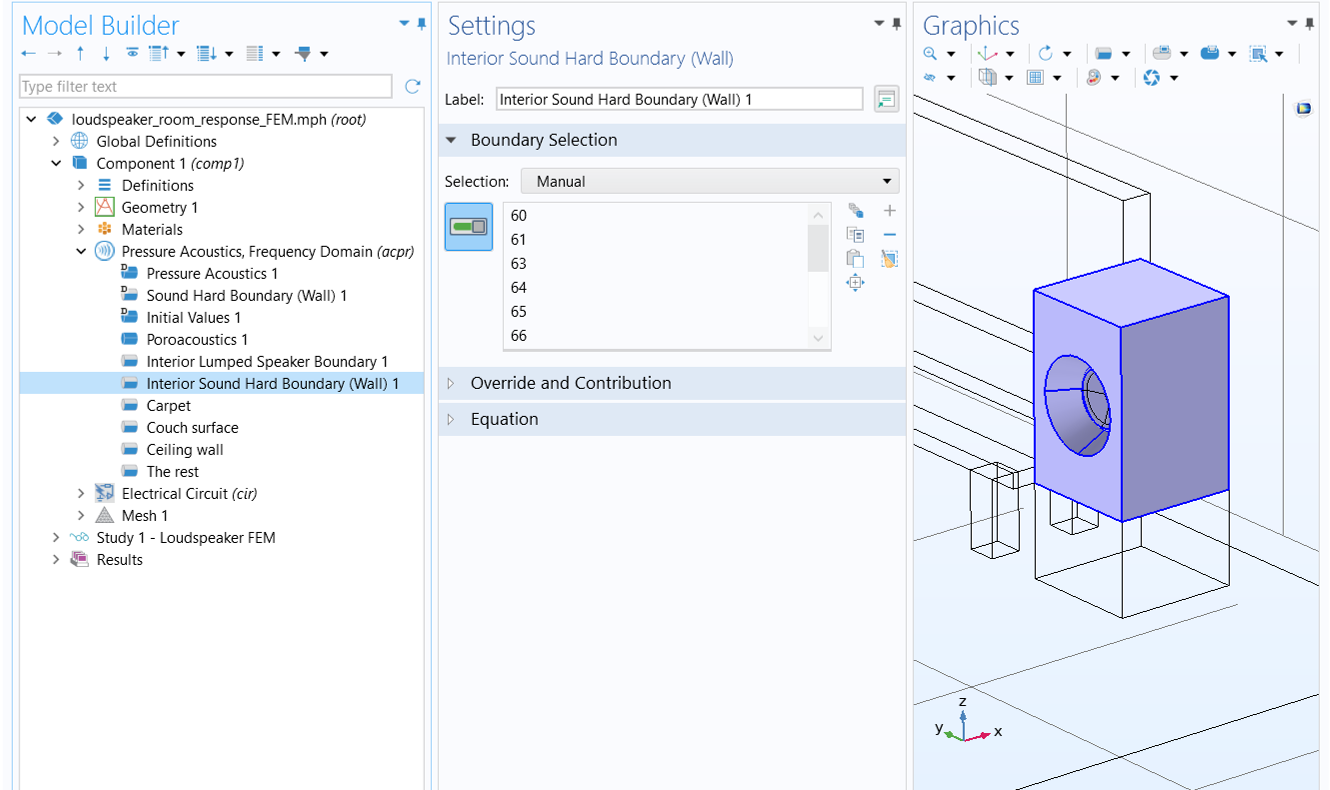
Next, add an Interior Lumped Speaker Boundary condition and apply it at the speaker diaphragm to model the loudspeaker using a lumped representation described in an Electrical Circuit interface, whereas the rest of the enclosure surfaces are modeled as sound hard walls by applying the Interior Sound Hard Boundary feature. Note that in the Speaker Geometry settings of the Interior Lumped Speaker Boundary node, the Speaker axis direction is set to (-1, 0, 0) to reflect the speaker's orientation in the negative x direction.  

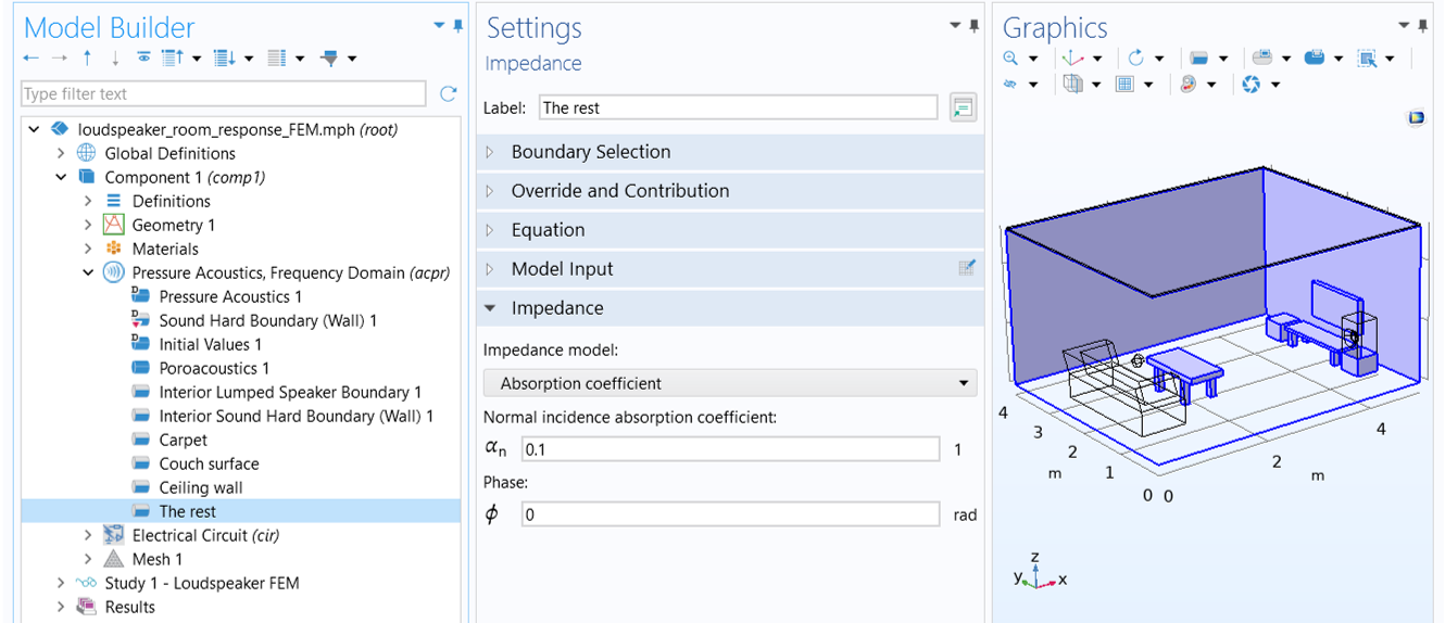
The furniture, TV and walls are not modeled explicitly, however, their surface properties are included to simulate sound reflection and absorption when waves hit them. In this example, we use several options provided by the Impedance boundary feature to model the acoustic behavior of the carpet, the couch, and the remaining surfaces. 

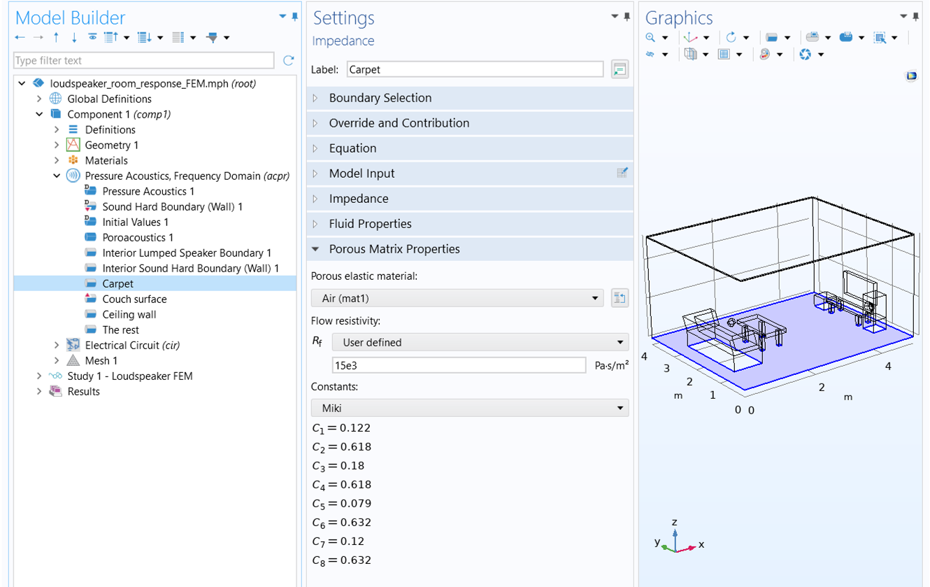
The Carpet

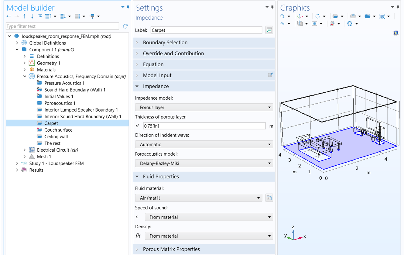
Sound absorption by the carpet is specified using the Porous layer impedance boundary condition, an alternative to explicitly modeling the porous layer with the Poroacoustics domain feature. This defines the carpet as a porous layer backed by a rigid, sound-reflective surface. Like the suspended ceiling, the Delany-Bazley-Miki poroacoustics model, with Miki's constants, is used to simulate the 0.75-inch thick carpet with a flow resistivity of 15×10³ Pa·s/m². Note that Automatic is selected for the Direction of incident wave, which automatically sets the angle of incidence to 50º behind the scenes. This angle provides an average value suitable for random incidence, making it particularly useful when modeling enclosed spaces like rooms.

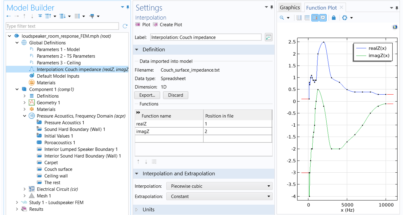
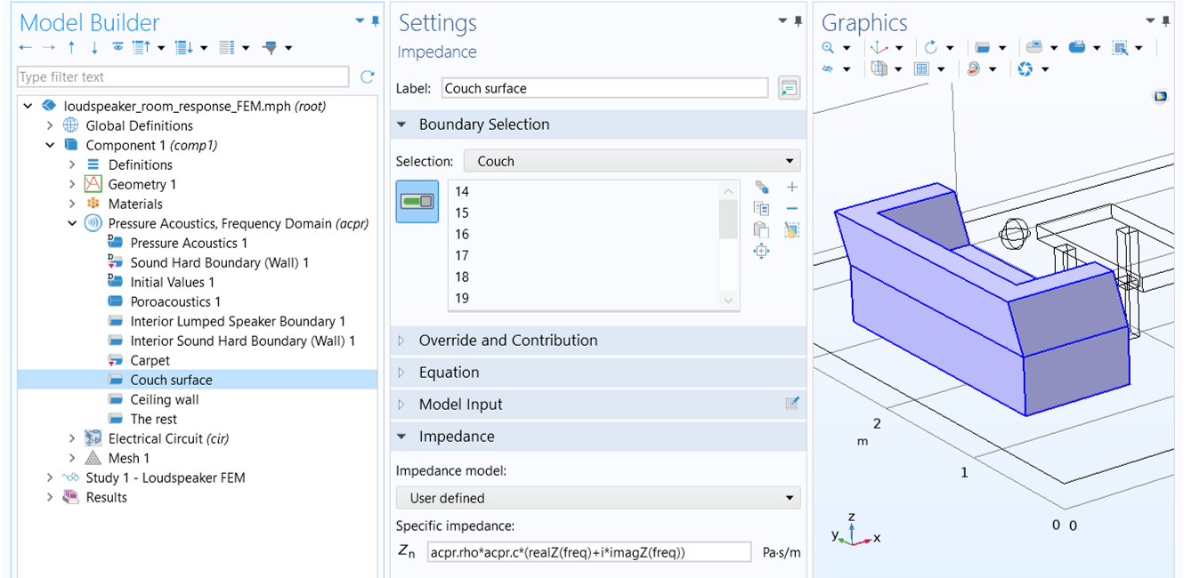
The Couch

The couch surfaces are described by another built-in impedance model, the User defined option, which allows for the input of frequency-dependent complex-valued impedance data to represent surfaces that are both resistive and reactive. This data can be sourced from measurements or derived from a sub-model solution. For demonstration purposes, we utilize data from the Car Cabin Acoustics - Frequency Domain Analysis tutorial, which incorporates acoustic impedance data for leather seats based on experimental values from Ref 1. The data is imported using interpolation functions under Global Definitions, as shown below. The imported impedance is the relative acoustic impedance, a dimensionless ratio comparing the impedance of leather seats to that of air. Consequently, to define the specific impedance, we multiply the relative acoustic impedance by the impedance of air.

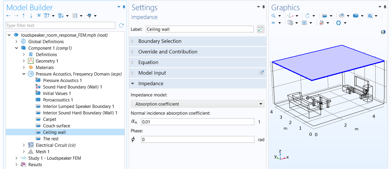
The Remaining Surfaces

For the remaining surfaces, we apply a constant absorption coefficient: 0.01 for the ceiling walls and 0.1 for the other surfaces.

The Lumped Speaker Model

A Thiele-Small (TS) representation of a circuit model is used here for the speaker driver. The TS parameters match those in the  Lumped Loudspeaker Driver  tutorial, discussed in detail in the "Using a Lumped Circuit Model" section of the "Modeling Speaker Drivers in COMSOL Multiphysics^®" course. These parameters are defined in a Parameters node under Global Definitions and are used to set up the Electrical Circuit interface.

The two way coupling between the circuit speaker model and the FEM acoustics model is completed by adding an External I vs. U  feature to the  Electrical Circuit  interface and setting the  Electric potential  to  Voltage from lumped speaker boundary, as shown in the image below. This setup takes the axial pressure force acting on the speaker diaphragm from the FEM acoustics model and incorporates it as a voltage source in the electrical circuit. 

The External I vs. U settings window using the voltage from the lumped speaker boundary. The lumped circuit model is coupled to the FEM acoustics model by an External I vs. U feature.

The Mesh

In this example, a single mesh is used, capable of resolving waves up to the highest study frequency of 1250 Hz. A finer mesh is applied to the receiver domain and diaphragm surfaces to capture the curvature in these areas. All domains are discretized using Free Tetrahedral elements, with the exception of the suspended ceiling and the air cavity behind it, where a Swept mesh is employed. The final mesh configuration is shown below. Please note that you also have the option to divide the frequency range into smaller bands and apply a different mesh for each band, as detailed in the blog post "How to Automate Meshing in Frequency Bands for Acoustic Simulations".

A very fine tetrahedral mesh covers all the surfaces in the model geometry. The mesh is generated to resolve waves up to 1250 Hz.

The Study

The coupled FEM-Circuit model is solved using a Frequency Domain study ranging from 50 Hz to 1250 Hz, with 10 Hz increments. The problem has approximately 10 million degrees of freedom (DOFs), which can be efficiently handled by the recommended iterative solver employing the Complex Shifted Laplacian (CSL or SL) method as a multigrid preconditioner. This approach generally enhances convergence speed for larger models. 

The physics and frequency range are defined for the study step. The Suggested Iterative Solver (Shifted Laplace) is used to solve the wave-based FEM model.

The Results

The images below display the sound pressure level distribution at four study frequencies: 50 Hz, 250 Hz, 500 Hz, and 1000 Hz. They provide information on the distribution of sound pressure levels and highlight the location of dead zones at each frequency. 

Four plots of a room using different frequencies show the sound pressure level with colored surface plots. Sound pressure level plots for four study frequencies.

The frequency domain study allows for the extraction of a transfer function from the speaker to any listening position. In this case, the averaged sound pressure level over the receiver surfaces is utilized to determine the frequency response captured by an omni-directional microphone, represented by the receiver sphere. 

The resulting frequency response, shown by the blue curve in the figure below, exhibits pronounced peaks and dips. These variations are influenced by several factors, including the total acoustic power radiated by the speaker, room modal resonances, frequency-dependent surface absorption, and frequency-dependent acoustic scattering. The same figure also displays the acoustic power radiated by the speaker as a red dotted line. Numerous peaks and dips in the sound pressure level curve closely correspond to those in the radiated power. Note that the effect of the acoustic load on the speaker is included in the model, which in turn influences the speaker’s output.  

A graph of the sound pressure level and radiated power associated with a range of frequncies. Sound pressure level measured at the receiver (blue solid curve) and acoustic power radiated by the speaker (red dotted line) as functions of frequency.

References:

1. P. Didier, “In situ estimation of the acoustic properties of vehicle interiors,” M.Sc. thesis, DTU Electrical Engineering (2019).