
拡散二重層
What Is the Double Layer?
In an electrolyte solution, ions are dissolved in a polar solvent, such as water. If there are more positive ions in a certain region of space than negative ions, then there will be a local positive space charge density. The diffuse double layer is a thin layer of electrolyte solution close to a charged surface, in which the solution acquires a local space charge density due to accumulation or depletion of the dissolved ions.
How Does the Diffuse Double Layer Form?
According to Coulomb's law, regions with a certain charge density repel ions of like charge and attract ions of opposite charge. Normally, this effect leads to electroneutrality, where the concentrations of positive and negative ions balance out locally, leaving no net charge density.
Let us consider a theoretical example. We can imagine an aqueous solution containing 10 mM hydrochloric acid (HCl) and 10 mM potassium chloride (KCl). In solution, these chemicals dissociate into three ions: solvated protons (H+), sodium (Na+) cations, and chloride (Cl-) anions. The concentrations of 10 mM H+, 10 mM K+, and 20 mM Cl- (half from acid and half from salt) add up to a net zero charge. Let us now imagine that the concentration of chloride is depleted at the right-hand side of a cell modeled in 1D. For example, an electrode might drive electrolysis to oxidize the chloride into chlorine gas that bubbles out of solution. Removing chloride ions will create extra positive charge density, which will repel both the H+ and K+ ions and attract oppositely charged Cl- ions so that electroneutrality is maintained.
The animation below shows 10 s of change in concentrations across a 0.5 mm distance from the surface where Cl- is depleted. For all points in space and time, the total space charge adds up to zero; that is, the sum of the H+ and K+ concentrations equals the Cl- concentration. Note that the K+ concentration is changed significantly, whereas the H+ concentration hardly changes. This is because the mobility of protons is much higher than the mobility of potassium ions. (See this page for the reasons why.) The majority of the current in the cell is then delivered by migration of the protons in an evolving electric field so that their concentration profile remains relatively unperturbed.
In the graph above, we observe electroneutrality over scales of hundreds of  and timescales of many seconds. Electroneutrality is violated, however, in the very close vicinity of a charged region, such as an electrode. When we place an electrolyte in contact with an electrical conductor, the conductor typically acquires a net surface charge, which can be altered by polarization of the electrochemical cell. Surface chemistry can give solids a net surface charge density too. For example, chemical modification of silica or carbon surfaces can alter the surface charge density.
The net charge on a surface — whether a conductor or a dielectric — is counterbalanced by a region of space charge in the solution, where ions of opposite charge to the surface are accumulated and ions of like charge to the surface are depleted. This layer is the double layer.
The schematic graph below shows the concentration profiles normal to a positively charged electrode. The concentration of the repelled cations is lowered close to the electrode surface; correspondingly, the concentration of the attracted anions is raised.
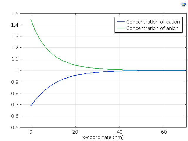
Cation and anion concentration profiles in a weak electrolyte close to a positively charged electrode surface.
Cation and anion concentration profiles in a weak electrolyte close to a positively charged electrode surface.
Note that this graph has scales of nm; it would be imperceptible in the animation above, where the x-scale is 1·104 times larger. In the next section we will investigate how to predict the spatial extent of the double layer.
Length and Time Scales in the Diffuse Double Layer
Let us consider a system containing diffuse mobile charges. The continuity equation for electrical charge gives

where  is the charge density (C/m3) and
  is the current density (A/m2).
Also, from Gauss's law, we have

where  is the permittivity of the medium (F/m) and
  is the electric field (V/m).
Consider the special case of an ohmic conductor, where the current density is linearly proportional to the electric field. Although this is not correct in all circumstances for an electrolyte, it is accurate in some limits and provides an instructive result. This special case gives

where  is the electrical conductivity (S/m).
Substituting into the continuity equation and treating conductivity and permittivity as constants, we can write a simple relation for the time evolution of the space charge density:

This is a first-order rate equation for the space charge density. The rate constant is the inverse of a characteristic charge dissipation time scale, given by the ratio of a solution's permittivity ( ) to conductivity ( ). The absolute permittivity of water is a little less than 10-9 F m-1, so for typical conductivities of electrolytes of the order of 1 S m-1, this time scale is of the order of nanoseconds.
Since electrical attractions and repulsions encourage the restoration of electroneutrality, the double layer only extends a very short distance away from a charged surface. The distance that the diffuse double layer extends is called the Debye length.
Many equations exist to define or derive the Debye length in terms of different properties. Here, let us consider the diffusion coefficient of the ions,  , and the characteristic charging time scale. The charge density is accumulated when the time scale for the transport of the ion to the charged surface is much smaller than the time scale for the dissipation of the charge density in the solution. This dissipation is due to ion attraction and repulsion. Using the Einstein relation to find the distance an ion can diffuse during the dissipation time scale, we have

Given that diffusion coefficients for ions in a solution are typically around 10-9 m2 s-1, we see that the Debye length usually takes a nanometer scale. Hence, the double layer — a region of permanent nonzero charge density in which electroneutrality is not maintained locally — typically extends only nanometers from a surface of fixed charge, such as an electrode or other solid surfaces. This justifies the use of electroneutrality in the prediction of the animation of the mixed HCl/KCl system shown in the figure above; it also explains why the double layer must be considered at nm length scales.
Equations Describing the Double Layer: Nernst–Planck–Poisson Equations
The electrostatic attraction and repulsion of ions at a charged surface can be described according to an electric field, which in turn corresponds to a certain potential difference, which is established across the double layer according to the charge that it screens. The amount of charge per unit potential difference gives the double-layer capacitance. Can this capacitance be predicted theoretically? Describing the diffuse double layer is a tightly coupled, nonlinear physical problem. This presents a challenge when using direct numerical simulation, which requires a flexible modeling approach.
Our starting point is Gauss's law (one of Maxwell's equations). In electrostatics, Gauss's law is used to relate charge density to voltage, and the same approach can be used here. Writing the electric field as the gradient of electric potential, we can express Gauss's law as

Here,  is the relative permittivity of the medium (about 80 for water at room temperature) and
  denotes electric potential (V).
The space charge density can be computed from the sum over all concentrations,  , of the ions (mol m-3), weighted according their charges,
  , and the Faraday constant (the absolute charge of a mole of electrons, ≈ 96485 F mol-1):

so

This equation has the overall mathematical form of a Poisson equation — an equation in which the Laplacian of the electric potential is equal to another function. It is common to combine this equation with the Nernst–Planck equations for the mass transport of each chemical species.
See What is Mass Transfer? and What is Ionic Migration? for further discussion of the origin and meaning of these equations.
For each species, we have

Overall, this gives a system of n + 1 equations for the n ion concentrations and the electric potential. These equations are called the Nernst–Planck–Poisson equations.
It is important to understand that the Nernst–Planck–Poisson equations are formulated for ideal solutions, i.e., infinitely dilute solutions. This condition is generally not true for ions in electrolyte solutions, and particularly not in double layers, where ions may accumulate to higher concentrations than in the bulk solution. Experimentally, ion–ion interactions and ion crowding are important phenomena that remain unconsidered in theories based on the Nernst–Planck equations. The refinement of double-layer theories is an active topic of academic research. Numerical methods still often begin from the Nernst–Planck–Poisson equations due to the relative simplicity and to provide guidance as a first approximation.
Solving the Nernst–Planck–Poisson Equations: Gouy–Chapman Theory
Although they represent a simplistic view of the double layer, the Nernst–Planck–Poisson equations are still highly nonlinear and difficult to solve. Analytical solutions exist only in very simple cases. When using numerical methods, it is essential to resolve the nanometer and nanosecond length and time scales described earlier by refining the:
- Discretization of the solution space
- The numerical time steps used for time-dependent problems
To build an understanding of the most important qualitative effects in the double layer, most theoretical models begin from the Gouy–Chapman theory (Ref. 1–2). In the Gouy–Chapman theory, the Nernst–Planck–Poisson equations are integrated using the following approximations:
- Steady-state conditions
- Pure binary electrolyte of one cation A+ and anion X-, each at fixed concentration
 far from the double layer
 - 1D geometry, for a double layer extending in the direction normal to an electrode, with the electrode dimensions much larger than the Debye length
- Fixed electric potential difference
 between the charged surface and bulk solution
At steady state, the Nernst–Planck equations can be written simply as

Considering that each ion takes a constant bulk concentration in the solution that is distant from the double layer, we can set  for the electroneutral exterior of the double layer and integrate to give

This is a Boltzmann equation, since it sets an equilibrium concentration for the ions at all points in space. Substituting this expression for each ion concentration into the space charge density in the Poisson equation gives

This is a second-order ordinary differential equation for the potential in the double layer. The high nonlinearity of the Poisson–Boltzmann equation set is made clear by the presence of the exponential term on the right-hand side. Due to its derivation, this equation is often called the Poisson–Boltzmann equation.
Under the abovementioned approximations, the Poisson–Boltzmann equation can be integrated. For small applied potentials (compared to RT/F), the result for the potential profile is as follows:

This means that the electric potential decays exponentially through the double layer. The decay length  is the Debye length, which in full can be written as

This mathematical result supports the expectation that the potential and concentration profiles in the double layer are only altered within a distance from the charged surface of the order of the Debye length.
One common extension to the Gouy–Chapman theory is the Gouy–Chapman–Stern (GCS) theory. This includes a description of the compact double layer at the electrode–electrolyte interface. This is the region of the double layer that lies inside the plane of closest approach of a solvated ion. Because the ions have finite size and are surrounded by water molecules, they cannot touch the electrode, but instead only approach up to a plane called the outer Helmholtz plane. Inside this plane, the capacitive response is described like a parallel plate capacitor, with an angstroms-thick layer of dielectric. Outside the outer Helmholtz plane, the ion concentrations vary in the region called the diffuse double layer.
The image below shows the potential profile in a typical double layer, plotted against distance from the charged surface in the unit of Debye length. Note that a part of the potential difference occurs within the compact double layer, located at x = 0 in this model. The remaining exponential profile decays over a few Debye lengths through the diffuse double layer.
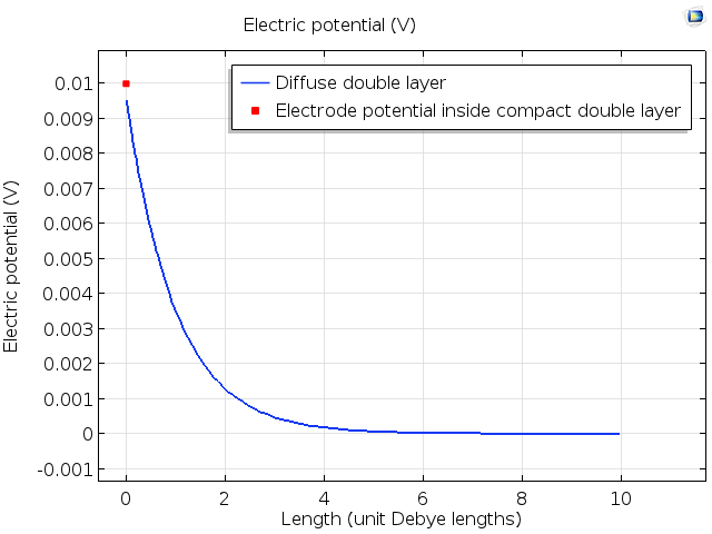
Unfortunately, neither the Gouy–Chapman–Stern theory or the numerical approaches based on the same approximations give general quantitative agreement with experiments. These theories give guidance for the important driving effects of the double layer, but many of their predictions are not replicated in practice. Even though the first major theories of the double layer date back to the turn of the 20th century, understanding the double layer more precisely is still an active area of research for theoretical electrochemists.
Double Layer Effects at the Macroscale: Electroosmosis
One example of a macroscale phenomenon created by the diffuse double layer is electroosmosis. In this effect, an applied electric field causes motion of the ions in the double layer. In turn, the ions drag the solvent with them because they remain solvated by water molecules. This has the effect of imparting a boundary stress or momentum to the fluid. Due to internal fluid friction (viscosity), the motion at the wall propagates into the bulk, causing an electroosmotic flow.
The magnitude of an electroosmotic flow can be defined according to an electroosmotic mobility, which is the ratio of the induced tangent flow velocity to the applied electric field. This means that

where  is the tangent component of electric field.
In turn, the electroosmotic mobility can be approximated in terms of the zeta potential,  , of the double layer (V), as

where  is the viscosity of the fluid (units Pa·s).
Here, the zeta potential is the potential difference across the diffuse double layer, between the outer Helmholtz plane and the bulk solution.
Devices Exploiting the Double Layer
Two examples of devices in which double-layer physics become important are supercapacitors and ion-sensitive field-effect transistors (ISFETs).
Supercapacitors are devices with very large capacitance; they can store a large amount of electrical energy at a given voltage. Supercapacitors are typically based on an electrochemical cell in which two electrodes with large surface area can be charged or discharged, as the ions in the electrolyte form a double layer adjacent to the electrode surfaces. In contrast to a battery, no direct electrochemical reaction takes place, so no electrons are exchanged between the chemical contents of the electrolyte and the external circuit; instead, current is drawn through the dynamic charging of a double layer. The high capacitance values of supercapacitors arise due to their very large surface areas, which are often realized through the use of highly porous materials, such as activated carbon.
In a normal metal–oxide–semiconductor field-effect transistor (MOSFET), a voltage is applied electrically to a gate electrode in order to control the flow of current between the source and drain electrodes in the semiconductor. In an ISFET, the metal electrode at the gate is replaced by a volume of electrolyte, in which the double layer at a solid surface controls the gate voltage. This gives the transistor sensitivity to properties of the electrolyte or the solid surface; for example, surface charge can be pH-sensitive due to protonation and deprotonation of surface groups.
Published: April 21, 2023References
- A.J. Bard and L.R. Faulkner, Electrochemical Methods: Fundamentals and Applications, 2nd ed., John Wiley & Sons, 2001.
- D.L. Chapman, "A Contribution to the Theory of Electrocapillarity," Philosophical Magazine, vol. 25, pp. 475–481, 1913.
- L.G. Gouy, Comptes Rendus Hebdomadaires des Séances de l’Académie des Sciences, vol. 149, pp. 654–657, 1909.
- O. Stern, "Zur Theorie Der Elektrolytischen Doppelschicht," Zeitschrift für Elektrochemie, vol. 30, pp. 508–516, 1924.
- "Supercapacitor", Wikipedia; https://en.wikipedia.org/wiki/Supercapacitor