In accordance with our Quality Policy, COMSOL maintains a library of hundreds of documented model examples that are regularly tested against the latest version of the COMSOL Multiphysics® software, including benchmark problems from ASME and NAFEMS, as well as TEAM problems.
Our Verification and Validation (V&V) test suite provides consistently accurate solutions that are compared against analytical results and established benchmark data. The documented models below are part of the COMSOL Multiphysics® software’s built-in Application Libraries. They include reference values and sources for a wide range of benchmarks, as well as step-by-step instructions to reproduce the expected results on your own computer. You can use these models not only to document your software quality assurance (SQA) and numerical code verification (NCV) efforts, but also as part of an in-house training program.
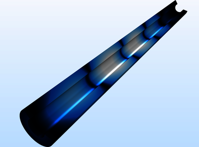
Simulation of Maxwell’s equations in the time domain is useful if the objective of the analysis is to observe a transient phenomenon, to find the time it takes a signal to propagate, or if the materials being modeled are non-linear with respect to the electric or magnetic field strength. ... 詳細を見る
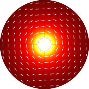
The coaxial cable (coax) is one of the most ubiquitous transmission line structures. It is composed of a central circular conductor, surrounded by an annular dielectric, and shielded by an outer conductor. This model computes the electric and magnetic field distribution inside of the ... 詳細を見る
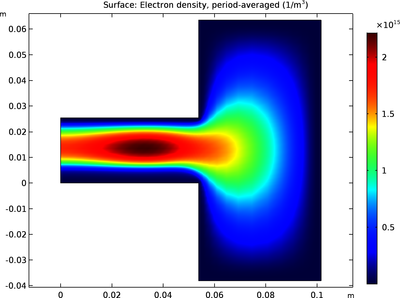
This model investigates the National Institute of Standards and Technology (NIST) Gaseous Electronics Conference (GEC) reference cell in two dimensions using the Plasma, Time Periodic interface. A 2D example helps in understanding the physics without excessive CPU time. The cell is ... 詳細を見る

This example benchmarks a NAFEMS validation model of a friction contact problem with an elastoplastic material model. A thin metal sheet is forced into a die by a punch. Both the compressing displacement and the release of the punch are modeled in order to compute the forming angle (at ... 詳細を見る
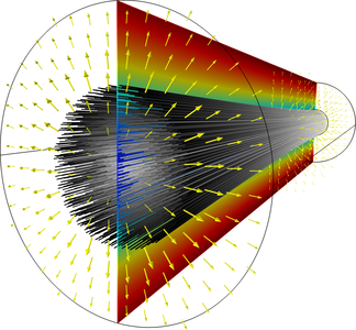
When modeling the propagation of charged particle beams at high currents, the space charge force generated by the beam significantly affects the trajectories of the charged particles. Perturbations to these trajectories, in turn, affect the space charge distribution. The Charged ... 詳細を見る
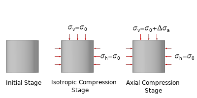
In this example, monotonic and cyclic triaxial tests are simulated using the Hardening Soil Small Strain material model. The model captures the effects of small strain stiffness and hysteresis under cyclic loading. The stress-strain relationship matches the hyperbolic curve reported in ... 詳細を見る
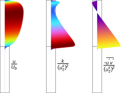
This setup demonstrates how the characteristics of turbulent flow in a channel are modified by the presence of an adjacent porous region. Asymmetric velocity profiles, higher turbulence levels, and higher friction coefficients both at the solid wall and the fluid-porous interface are ... 詳細を見る
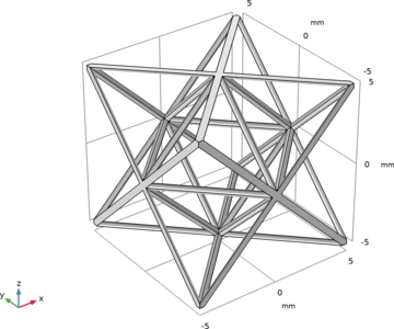
Lattice materials enable the creation of advanced additive manufacturing materials with customized mechanical properties. At the macroscopic level, these heterogeneous materials can be modeled as homogeneous materials. Homogenization techniques can accurately determine the material's ... 詳細を見る

This model represents a test case of a flow in an elastic tube which is present in several applications. This specific case models viscoelastic flow and represents steady flow in a channel in which part of the upper wall is replaced by an elastic plate subjected to an external pressure. ... 詳細を見る

This model illustrates the instability of a space arc frame under concentrated vertical loading. The Beam interface is utilized. Two different approaches are used: A full incremental nonlinear analysis, where a small lateral load is applied to break the symmetry of the structure A ... 詳細を見る