電気めっきモジュールアップデート
COMSOL Multiphysics® バージョン 6.4 では, 電気めっきモジュールをご利用のユーザー向けに, 水性電解質をモデリングするためのインターフェース, エネルギー損失を評価するためのパワー損失変数, および充放電負荷サイクルを定義する新機能が導入されました. これらのアップデートやその他の詳細については, 以下をご覧ください.
水性電解質輸送
弱酸, 弱塩基, 両性イオン, および一般的な複合種を特徴とする水性電解質のモデリング, ならびに機構論的腐食モデリング, 生物系の電気化学モデル, 電気化学センサーモデリングなどの用途向けに, 新しい 水性電解質輸送 インターフェースが追加されました. これは, 希薄水性電解質中の電位および化学種の濃度場を計算します. この輸送は, 拡散, マイグレーション, 対流に加え, 電気中性と水の自己イオン化平衡反応 (自己プロトロシス) を組み込んだネルンスト・プランク方程式によって定義されます. 方程式反応のより効率的な処理とモデル設定の容易さから, この新しいインターフェースは, より汎用的な 3次電流分布 (ネルンスト・プランク) インターフェースよりも, 使用が適当な場合があります.
パワー損失評価変数
電気化学 インターフェースに新たに導入されたパワー損失変数を使用することで, 電池セルにおける総パワー損失の大きさを評価し, セパレータ, 電極, 電流導体などの個々の構成要素間の損失を比較することが可能になりました. これらの変数は, 充電・放電負荷サイクル下での電池セルの往復エネルギー効率を, 時間経過に伴うパワー損失を積分することで計算するのにも使用できます.
パワー損失は, 反応および輸送される全物質のギブズ自由エネルギーの損失に基づいて定義され, オーム損失, 濃度損失, 活性化損失を区別することができます. 粒子挿入をサポートする電池インターフェースでは, 個別の挿入輸送損失変数も定義されます. これらの変数は, ドメインおよび境界上でローカルな値として, セル全体にわたる積分値として, もしくは個々のモデルツリーノードごとの値として利用可能です. 各損失メカニズム (オーム損失, 活性化損失, 輸送損失) の過電圧寄与は, 総電流で除算することで計算できます.

負荷サイクル
複雑なサイクル設定の簡便なセットアップを可能にするため, ほとんどの 電気化学 インターフェースに新たな 負荷サイクル 機能が追加されました. この機能を使用すると, 電圧, パワー, 電流, C レート, 休止 ステップを任意の順序で追加し, 任意の充放電負荷サイクルを定義できます. 負荷サイクルの各ステップでは, 時間, 電圧, 電流の制限値, および任意の変数式を用いたユーザー定義条件に基づく, 1つまたは複数の動的継続/中断 (切り替え) 基準を定義できます. 多様な負荷サイクル定義オプションに加え, この新機能では電流・電圧プローブの自動定義やソルバー停止条件の設定も可能です.
サブループ サブ機能を使用すると, 例えば, 長期の充放電サイクル試験と基準性能試験を組み合わせて実施することができます. なお, パワー および サブループ サブ機能は, バッテリデザインモジュールおよび燃料電池 & 電解槽モジュールでのみご利用いただけます.

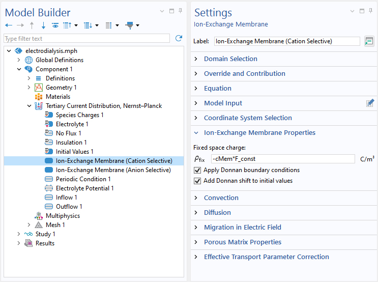
イオン交換膜モデルの自動初期化
電気的中性とドナン平衡の遵守のため, 3次電流分布 (ネルンスト・プランク) インターフェースの イオン交換膜 機能に 初期値に Donnan シフトを追加 オプションが追加されました. このオプションは, 有効な イオン交換膜 ドメインノードの初期値機能で指定された初期濃度および電位値を自動的にシフトします. これは, ユーザー定義値が膜と平衡状態にあるバルク液体電解質の値を表すと仮定しています. シフトされた初期値はソルバーの初期値として使用されます. このオプションを有効にすると, 追加の解析ステップで膜の固定空間電荷を所定の非ゼロ値までスイープする必要がなくなるため, モデル設定が簡略化されます. この機能は電気透析セルでの脱塩チュートリアルモデルでご覧いただけます.
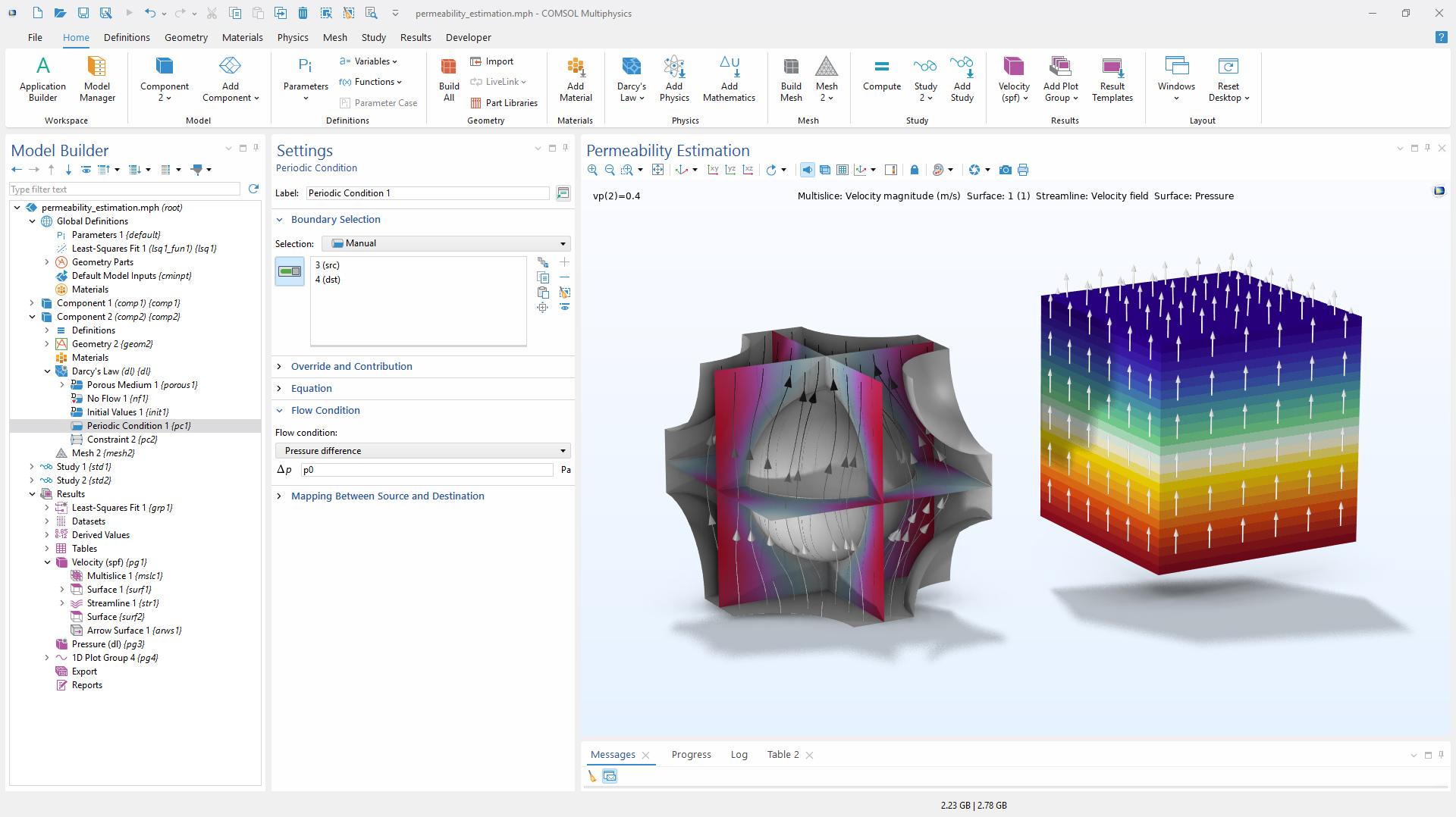
周期条件
ダルシー則 および リチャーズ方程式 インターフェースに新たな 周期条件 機能が追加され, 2つ以上の境界間の流れに対して周期性を容易に強制できるようになりました. さらに, 圧力ジャンプを直接指定するか, 質量流量を規定することで, ソース境界と行先境界間に圧力差を生成することが可能です. 周期条件は, 代表体積要素のモデル化や, 均質化された多孔質媒体の有効特性の計算に一般的に用いられます.
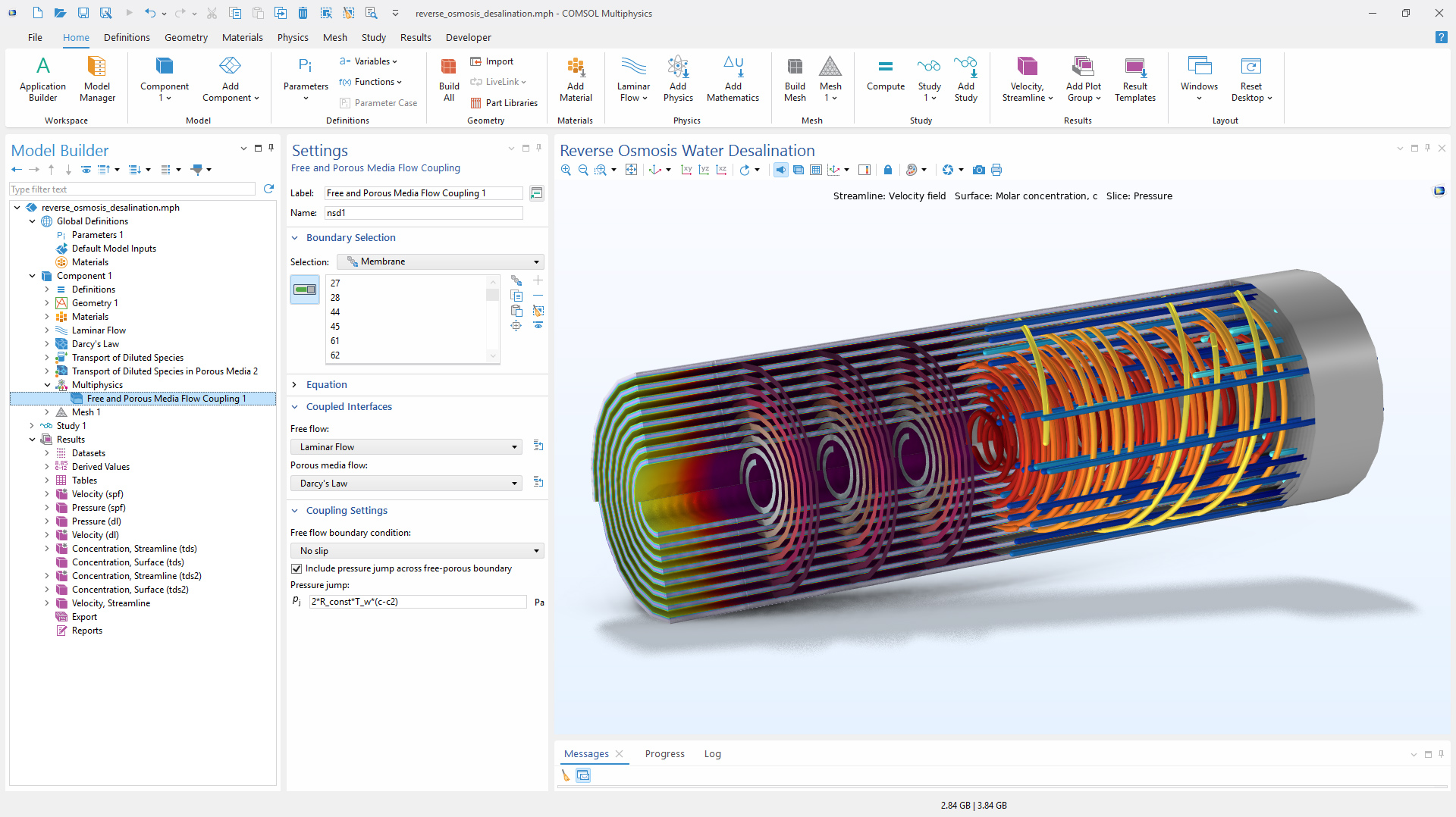
自由および多孔質流れカップリングにおける圧力ジャンプオプション
自由および多孔質流れカップリング には, 自由媒体と多孔質媒体の境界における圧力ジャンプを考慮する新オプションが追加されました. これにより, 例えば多孔質スペーサー材料で支持された半透膜における浸透圧や, 多相流における毛管圧力による圧力ジャンプなどのモデル化が可能になります.
更新されたチュートリアルモデル
COMSOL Multiphysics® バージョン 6.4 では, 電気めっきモジュールのチュートリアルモデルが更新されました.
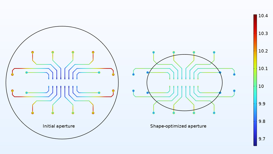
プリント基板の電気めっきにおけるアパーチャ形状最適化